SpatiaLite Cookbook Chapter 04: Haute cuisine

SELECT
 rw.name AS Railway,
 c.community_name AS Community,
 p.province_name AS Province,
 r.region_name AS Region
FROM railways AS rw
JOIN communities AS c ON
(
 -- 1st filter: Railway-line (MULTILINESTRING) going through BoundingBox of Community [MULTIPOLYGON]
 c.ROWID IN
 (
  SELECT ROWID FROM SpatialIndex WHERE
  (
   -- the BoundingBox is a square 1000 meters around the Populated-Place (width/height 2000 meters)
   (f_table_name = 'communities') AND
   -- geometry-column to use (only mandatory when the TABLE contains more than 1 geometry)
   (f_geometry_column = 'geometry') AND
    -- to calculate the values precisely, transform Railway-Line from 23032 to 32632
   (search_frame = BuildMbr(795201.2499,4625100.7198,811621.7722,4615838.1497,32632))
  )
 ) AND
 ST_Intersects
 (
  -- Does the Railway-Line pass through ...
  ST_Transform
  (
   -- transform from 'ED50 UTM zone 32' to 'WGS 84 / UTM zone 32N'
   rw.geometry,32632
  ),
  -- ... the wiggly boundry of the Community ?
  c.geometry
 )
)
JOIN provinces AS p ON (p.province_id = c.province_id)
JOIN regions AS r ON (r.region_id = p.region_id)
ORDER BY r.region_name, p.province_name, c.community_name;
-- 6 records

We now get our expected result (Marino is now out of range):

Railway	Community	Province	Region
Ferrovia Roma-Napoli	Aprilia	Latina	Lazio
Ferrovia Roma-Napoli	Ardea	Roma	Lazio
Ferrovia Roma-Napoli	Lanuvio	Roma	Lazio
Ferrovia Roma-Napoli	Pomezia	Roma	Lazio
Ferrovia Roma-Napoli	Roma	Roma	Lazio
Ferrovia Roma-Napoli	Velletri	Roma	Lazio

Well, ... almost the expected result

Further south (outside of the image) the Railway-Line runs into Velletri,
which can be seen at the right edge, and was overlooked when the images were made.

And with that we complete 'Brilliant idea (version 2)' with no 'Brilliant idea (version 3)' being planned.

---

Since the goal is to identify any Populated-Place laying within a given distance radius of: 1, 2.5, 5, 10 and 20 KM

a Populated-Place outside the BoundingBox, but inside the given radius must also be found.

---

For this we will extend the original search_frame of the SpatialIndex from:

• ST_Transform(rw.geometry,32632)

to:

• ST_Buffer(ST_Transform(ST_Envelope(rw.geometry),32632), radius)

---

Achieved optimations:

• ST_Envelope will return 5 POINTs of the BoundingBox of the Railway-Line,

  since the SpatialIndex only uses the BoundingBox of a geometry anyway

• ST_Transform will transform these 5 POINTs (instead of the > 1000 POINTs contained the Roma-Napoli Railway-Line)
• ST_Buffer will increase the area of the BoundingBox by the given radius

The SpatialIndex will return more results this way, but the results will be more realistic than the previous version.

and now, (... da,da,da,daaa ...) presenting the horror Query in all it's glory:
   (but don't worry - each portion will be explained further down)

SELECT
 rw.name AS Railway,
 pp_e.name AS PopulatedPlace,
 ST_Distance(ST_Transform(rw.geometry, 32632),pp_e.geometry) AS "distance [in meters]",
 (ST_Distance(ST_Transform(rw.geometry, 32632),pp_a.geometry) <= 1000.0) AS "A class [< 1Km]",
 (ST_Distance(ST_Transform(rw.geometry, 32632),pp_b.geometry) > 1000.0) AS "B class [< 2.5Km]",
 (ST_Distance(ST_Transform(rw.geometry, 32632),pp_c.geometry) > 2500.0) AS "C class [< 5Km]",
 (ST_Distance(ST_Transform(rw.geometry, 32632),pp_d.geometry) > 5000.0) AS "D class [< 10Km]",
 (ST_Distance(ST_Transform(rw.geometry, 32632),pp_e.geometry) > 10000.0) AS "E class [< 20Km]"
FROM railways AS rw
JOIN populated_places AS pp_e ON
(
 -- retrieve 'E class' Populated-Places using the SpatialIndex
 pp_e.id IN
 (
  SELECT ROWID FROM SpatialIndex WHERE
  (
   -- only Populated-Places within the BoundingBox of the Railway-Line [909=818+91]
   (f_table_name = 'populated_places') AND
   -- geometry-column to use (only mandatory when the TABLE contains more than 1 geometry)
   (f_geometry_column = 'geometry') AND
   -- extract BoundingBox from Railway-Line ; Tranform result and expand by 20000.0 meters
   (search_frame = ST_Buffer(ST_Transform(ST_Envelope(rw.geometry),32632), 20000.0))
  )
 ) AND
 -- check if candidates are within the distance condition [376, NOT=533]
 (ST_Distance(ST_Transform(rw.geometry, 32632),pp_e.geometry) <= 20000.0)
)
LEFT JOIN populated_places AS pp_d ON
(
 (pp_e.id = pp_d.id) AND
 -- retrieve 'D class' Populated-Places using the SpatialIndex
 pp_d.id IN
 (
  SELECT ROWID FROM SpatialIndex WHERE
  (
   -- only Populated-Places within the BoundingBox of the Railway-Line [909=818+91]
   (f_table_name = 'populated_places') AND
   -- geometry-column to use (only mandatory when the TABLE contains more than 1 geometry)
   (f_geometry_column = 'geometry') AND
   -- extract BoundingBox from Railway-Line ; Tranform result and expand by 10000 meters
   (search_frame = ST_Buffer(ST_Transform(ST_Envelope(rw.geometry),32632), 10000.0))
  )
 ) AND
 -- check if candidates are within the distance condition
 (ST_Distance(ST_Transform(rw.geometry, 32632),pp_d.geometry) <= 10000.0)
)
LEFT JOIN populated_places AS pp_c ON
(
 (pp_d.id = pp_c.id) AND
 -- retrieve 'C class' Populated-Places using the SpatialIndex
 pp_c.id IN
 (
  SELECT ROWID FROM SpatialIndex WHERE
  (
   -- only Populated-Places within the BoundingBox of the Railway-Line [909=818+91]
   (f_table_name = 'populated_places') AND
   -- geometry-column to use (only mandatory when the TABLE contains more than 1 geometry)
   (f_geometry_column = 'geometry') AND
   -- extract BoundingBox from Railway-Line ; Tranform result and expand by 5000 meters
   (search_frame = ST_Buffer(ST_Transform(ST_Envelope(rw.geometry),32632), 5000.0))
  )
 ) AND
 -- check if candidates are within the distance condition
 (ST_Distance(ST_Transform(rw.geometry, 32632),pp_c.geometry) <= 5000.0)
)
LEFT JOIN populated_places AS pp_b ON
(
 (pp_c.id = pp_b.id) AND
 -- retrieve 'B class' Populated-Places using the SpatialIndex
 pp_b.id IN
 (
  SELECT ROWID FROM SpatialIndex WHERE
  (
   -- only Populated-Places within the BoundingBox of the Railway-Line [909=818+91]
   (f_table_name = 'populated_places') AND
   -- geometry-column to use (only mandatory when the TABLE contains more than 1 geometry)
   (f_geometry_column = 'geometry') AND
   -- extend the search_frame by 2500 meters ('Roma, Foro Romano' will be found)
   (search_frame = ST_Buffer(ST_Transform(ST_Envelope(rw.geometry),32632), 2500.0))
  )
 ) AND
 -- check if candidates are within the distance condition
 (ST_Distance(ST_Transform(rw.geometry, 32632),pp_b.geometry) <= 2500.0)
)
LEFT JOIN populated_places AS pp_a ON
(
 (pp_b.id = pp_a.id) AND
 -- retrieve 'A class' Populated-Places using the SpatialIndex
 pp_a.id IN
 (
  SELECT ROWID FROM SpatialIndex WHERE
  (
   -- only Populated-Places within the BoundingBox of the Railway-Line [909=818+91]
   (f_table_name = 'populated_places') AND
   -- geometry-column to use (only mandatory when the TABLE contains more than 1 geometry)
   (f_geometry_column = 'geometry') AND
   -- extract BoundingBox from Railway-Line ; Tranform result and expand by 1000 meters
   (search_frame = ST_Buffer(ST_Transform(ST_Envelope(rw.geometry),32632), 1000.0))
  )
 ) AND
 -- check if candidates are within the distance condition
 (ST_Distance(ST_Transform(rw.geometry, 32632),pp_a.geometry) <= 1000.0)
)
ORDER BY PopulatedPlace;
-- 512 records [00:00:05.022]

Yes, this one really looks like a complex and intimidating query, but it is not as bad as it looks.

---

You already know the trick:
   you simply have to break down the Sql-Query into several smaller chunks.

And then you'll soon discover that each chunk is quite a simple affair.

---

Let us examine this then, piece by piece:

Chunk 1: the outer chunk
   (like the outer crust of a pie)

SELECT
 rw.name AS Railway, ...
FROM railways AS rw
JOIN populated_places AS pp_e ON (...)
LEFT JOIN populated_places AS pp_d ON (...)
LEFT JOIN populated_places AS pp_c ON (...)
LEFT JOIN populated_places AS pp_b ON (...)
LEFT JOIN populated_places AS pp_a ON (...);

• we'll simply JOIN the 'railways AS rw' and the 'populated_places AS pp_e' tables togeather
     and there is nothing strange in that, is there ?
• then we'll perform a LEFT JOIN of the populated_places AS pp_d table a second time:
     and you'll, no doubt, remember that a LEFT JOIN inserts a valid row into the result-set even when the right-sided term evaluates to NULL, right?
• and finally we'll simply repeat LEFT JOIN for pp_c, pp_b and pp_a.

---

Chunk 2 a: part of the inner chunk
   (an ingredient inside the crust of a pie)

Defining each JOIN (or LEFT JOIN)

We'll obviously start by using the SpatialIndex, which will, fast and efficiantly extract all of the likley candidates that will fulfill the distance criteria.
   (what will be used as the main ingredient of the pie  (mincemeat for a meat pie, peakan's for sweet pie, or something else, whatever might be needed for a vegatarian)

...
JOIN populated_places AS pp_e ON
(
 -- retrieve 'E class' Populated-Places using the SpatialIndex
 pp_e.id IN
 (
  SELECT ROWID FROM SpatialIndex WHERE
  (
   -- only Populated-Places within the BoundingBox of the Railway-Line [909=818+91]
   (f_table_name = 'populated_places') AND
   -- geometry-column to use (only mandatory when the TABLE contains more than 1 geometry)
   (f_geometry_column = 'geometry') AND
   -- extract BoundingBox from Railway-Line ; Tranform result and expand by 20000 meters
   (search_frame = ST_Buffer
                   (
                    -- to calculate the values precisely, transform Railway-Line from 23032 to 32632
                    ST_Transform
                    (
                     -- Extract the BoundingBox of the geometry (which is all the SpatialIndex uses)
                     ST_Envelope
                     (
                      -- the geometry to use for Envelope/Transform and Buffer
                      rw.geometry
                     ),
                      --the SRID to transform the geometry to
                     32632
                    ),
                    --Expand by value in SRID-Units (for 32632: meters)
                    20000.0
                   )
   )
  )
 ) AND ...
)

---

Chunk 2 b: also a part of the inner chunk
   (to further the flavor the main ingredient inside the pie like onions, syrup or (again) what ever else is needed)

Evaluate, with ST_Distance the candidates, checking if this one falls within the expected threshold for the corresponding Class.

 ... AND
 (ST_Distance(ST_Transform(rw.geometry, 32632),pp_e.geometry) <= 20000.0)

---

Chunks 2 c-z: any other conditions, as needed.
   (anything else to make the pie nice and tasty)

---

With that, the main building block of the query should be clear:

• the first JOIN will include into the result-set any Populated Place falling within 20 Km from the railway line.
• any other LEFT JOIN will then test decreasing distances, accordingly to the imposed Class boundaries.
• and each LEFT JOIN carefully checks if the Populated Place ID is the same of the previous successfully identified Class, as in: pp_d.id = pp_c.id
• each time one such LEFT JOIN will fail, then corresponding NULL-values will be inserted into the result-set.

Everything else ... is a repetition of each Chunks N a-z for the other classes.
   ( ... is making enough pies for a nice party. Don't forget the vegatarian though,  there is always one that turns up ! Remember: in 50 years, it may be the other way around.)

---

And now you are ready to start experimenting ...

by making further changes to this query like

• adding some other ORDER BY
• adding/changing some new WHERE conditions

Soon you will see how easy and powerful is really is.

---

• Don't be discouraged if doesn't work the first ... fourth time off !
• Remember: Rome wasn't built in a day !
• Things of quality take their time to evolve.

---

by 'playing around' with your borrowed recipies by

• adding some other ingredients
• adding/changing some new spices for more flavors

Soon you will see how a bit of creativity can make a big difference (enough not to notice that ...).

---

• Don't be discouraged if tasts horrable the first ... fourth time off !
• Remember: Italian cooking started before and continued after, Marco Polo's visit to foreign parts !
• Things of quality take their time to evolve.

• as usual, we'll first create the table, omitting any Geometry column
• and we'll then create the Geometry column in a second time, using AddGeometryColumn(); but you already known all this.
• placing this new table into the 32632 SRID [WGS 84 / UTM zone 32N] is an absolutely obvious choice: after all, the original railways table is into the same identical SRID
• declaring a MULTYPOLYGON Geometry type is less obvious: but we'll see later why this is required.

---

CREATE TABLE railway_zones
(
 id INTEGER NOT NULL PRIMARY KEY AUTOINCREMENT,
 railway_name TEXT NOT NULL,
 zone_name TEXT NOT NULL
);

SELECT
 AddGeometryColumn('railway_zones', 'geometry', 32632, 'MULTIPOLYGON', 'XY');

---

Nothing new in this INSERT INTO ... SELECT ... statement (having allready been done before).

INSERT INTO railway_zones
(id, railway_name, zone_name, geometry)
 SELECT
  NULL, name,
  'A class [< 1Km]' AS zone_name,
  CastToMultiPolygon
  (
   ST_Buffer(ST_Transform(geometry,32632), 1000.0)
  ) AS geometry
 FROM railways;

Except for the following points:

• we'll use ST_Buffer() to create a POLYGON corresponding to the 1Km A-class zone.
• Please note: since the exact type of any Geometry created by ST_Buffer(); may differ:
     either this function will create a POLYGON, or a MULTIPOLYGON depending on the exact shape of the input line,
     but also influenced by the given buffer radiusas well.
• so, in order to avoid any possible type inconsistency we defined a MULTIPOLYGON Geometry for this table.
• and we are now forcing the type by calling the explicit type-casting function CastToMultiPolygon()
• since the source geometry uses SRID 23032, 'ED50 UTM zone 32', ST_Transform must be used.

---

Note:
   Adding a 'AS column_name' ist strictly cosmetic (not mandatory),
    but sometimes useful for clarity (which column is intended in the SELECT statement)

Creation of the TABLE admin_regions

Now you'll create and populate the admin_regions table:

-- this can take some time [ST_Area, ST_Union etc.], start TRANSACTION
BEGIN;
-- not being the first version of our masterpiece, remove previous version
DROP TABLE IF EXISTS admin_regions;

---

CREATE TABLE admin_regions
(
 id_region INTEGER NOT NULL PRIMARY KEY,
 name_region TEXT NOT NULL,
 -- Population of Region, as whole persons
 population_region INTEGER DEFAULT 0,
 -- Area of Region, in meters
 area_region DOUBLE DEFAULT 0,
 -- Amount of Cities belonging to the Region,
 city_count INTEGER DEFAULT 0,
 -- Amount of Provinces belonging to the Region,
 province_count INTEGER DEFAULT 0,
 -- id of Country the Region belongs to [default: 39, Italy]
 id_country INTEGER DEFAULT 39,
 -- name of Country the Region belongs to [default: Italy]
 name_country TEXT DEFAULT 'Italy'
);

---

SELECT
 AddGeometryColumn('admin_regions', 'geom_region', 32632, 'MULTIPOLYGON', 'XY');

---

INSERT INTO admin_regions
(id_region, name_region, population_region, area_region, city_count, province_count, geom_region)
SELECT
 id_region,
 name_region,
 -- Population of Region, as whole persons
 sum(population_province) AS population_region,
 -- Area of Region, in meters
 ST_Area(ST_Union(geom_province)) AS area_region,
 -- Amount of Cities belonging to the Region,
 sum(city_count) AS city_count,
 -- Amount of Provinces belonging to the Region,
 count(id_province) AS province_count,
 -- default values for id_country[39] and name_country['Italy']
 -- Build outer Boundry of Region, based on Province-Geometries and stored as MULTIPOLYGON
 CastToMultiPolygon(ST_Union(geom_province)) AS geom_region
FROM admin_provinces
 -- needed for aggregate functions: sum, count, ST_Area and ST_Union
GROUP BY id_region;

---

-- end TRANSACTION
COMMIT;

• as in the previous step you'll use ST_Union() and GROUP BY to aggregate regions Geometries.
• please note well: in this example you have explicitly created the regions table, then using AddGeometryColumn() so to create the regions.geometry column.
  And finally you have used INSERT INTO ... (...) SELECT ... in order to populate the table.
  The procedure is different, but the final result is exactly the same one as in the previous example.

SELECT
 id_region,
 name_region,
 population_region,
 area_region,
 city_count,
 province_count,
 geom_region
 -- We assume that [39, Italy] is known
FROM admin_regions;

Just a quick check ...

id_region	name_region	population_region	area_region	city_count	province_count	geom_region
1	Piemonte	4363916	25386696893.947697	1206	8	BLOB sz=258069 GEOMETRY
2	Valle D'Aosta	4363916	3260854219.911026	74	1	BLOB sz=57837 GEOMETRY
3	Lombardia	9704151	23863097447.125397	1544	12	BLOB sz=296140 GEOMETRY
...	...	...	...	...	...	...

And then you can display the admin_regions map layer using QGIS.

      Advanced Topic  :

Beware that: this topic is of a more  advanced  nature.
You may want to look into this later.
The information here in not strictly needed at this point.

---

Goals:
  Background:
    The Italian Peninsula contains 3 countries

• Italian Republic (since 1861-03-17 as unified country)
• San Marino (since 0301-09-03 as Republic)
• Vatican City (since 1929-02-11 City-State through the 'Lateran Treaty' agreement)

    The Italian National Census 2011 data does not reference San Marino or the Vatican City as a Region, Province or City
    They are, however, indirectly contained in the data since both are enclaves of the Italian Republic.

The goals will therefore be:

• extract both enclaves from the existing data
• add each enclave to the admin_regions table, with an country definition
• dynamically create as country in the admin_countries table, togeather with Italy

Notes:
  Most projects will contains aspects, which cannot be resolved within a general solution.
  Often one time solutions must be delt with.
  Also each aspect, may need a different solution.
  Some aspects, there may be different methods for a solution.

All of these are true for the case of the 2 enclaves:

• the method for the Vatican City cannot be used for San Marino
• there is more that one method to resolve the San Marino 'problem'

The Vatican City

---

Explanation of Image: Area Rome (1748, Nuova Topografia di Roma di Giovanni Battista Nolli)

• The Community boundry (yellow) of Roma (id_city=58091)
• The Province boundry (blue) of Roma (id_province=58)
• The Region boundry (red) of Roma (id_region=12)

---

The Community of Rome as seen in Blob-Explorer:

An Sql-Query to analyse the geometry and work out the information needed later for the INSERT command.
Notes:
  the numbers seen in the Blob-Explorer can be used for the ST_GeometryN and ST_InteriorRingN commands.
  each POLYGON is shown as 'exterior ring' n the Blob-Explorer

SELECT
 -- Select the Community of Rome and view in Blob-Explorer
 geom_city,
 -- How many Polygons does the Community of Rome have ?
 ST_NumGeometries(geom_city) AS num_geom_city,
 -- Select the first Polygon [1 based]
 ST_GeometryN(geom_city,1) AS first_geom_city,
 -- How many Interior-Rings does the first Polygon have ?
 ST_NumInteriorRing(ST_GeometryN(geom_city,1)) AS num_InteriorRing,
 -- Select the first Interior-Ring of the first Polygon [1 based]
 ST_InteriorRingN(ST_GeometryN(geom_city,1),1) AS linestring_Vatican_City,
 -- Convert the Interior-Ring (closed LINESTRING) to a Polygon
 ST_MakePolygon(ST_InteriorRingN(ST_GeometryN(geom_city,1),1)) AS polygon_Vatican_City,
 -- Convert the Polygon to am MULTIPOLYGON for the admin_regions TABLE
 CastToMulti(ST_MakePolygon(ST_InteriorRingN(ST_GeometryN(geom_city,1),1))) AS multi_polygon_Vatican_City,
 -- Select the third Polygon [1 based]
 ST_GeometryN(geom_city,3) AS third_geom_city,
 -- Area of the third Polygon [142.236898 meters]
 St_Area(ST_GeometryN(geom_city,3)) AS third_geom_city_area,
 -- Select the fourth Polygon [1 based]
 ST_GeometryN(geom_city,4) AS fourth_geom_city,
 -- Area of the fourth Polygon [81.987090 meters]
 St_Area(ST_GeometryN(geom_city,4)) AS fourth_geom_city_area,
 -- Select the fifth Polygon [1 based]
 ST_GeometryN(geom_city,5) AS fifth_geom_city,
 -- Area of the fifth Polygon [34.695557 meters]
 St_Area(ST_GeometryN(geom_city,5)) AS fifth_geom_city_area,
 -- Create a corrected version of the Community of Rome geometry
 ST_Collect
 (
  -- Select the first Polygon [1 based]
  ST_GeometryN(geom_city,1),
  -- Select the second Polygon [1 based]
  ST_GeometryN(geom_city,2)
 ) AS corrected_geom_city
FROM admin_cities
WHERE
(
 (id_city=58091)
);

Conclusions:

• multi_polygon_Vatican_City shows the Boundry of the Vatican City as we need it
• POLYGONs: 3,4,5 are candidates for the catagory 'goofups'
• corrected_geom_city could be used to correct the faulty Community of Rome geometry

---

INSERT Sql: the Vatican City

INSERT INTO admin_regions
(id_region, name_region, population_region, area_region, city_count, province_count, id_country, name_country, geom_region)
 SELECT
  -- County calling (telephon) code
  387 AS id_region,
  'Stato della Città del Vaticano (Status Civitatis Vaticanae)' AS name_region,
  -- Population of Region, as whole persons [wiki data]
  829 AS population_region,
  -- Area of Region, in meters [528986.602061 ; wiki: 301340]
  ST_Area(ST_MakePolygon(ST_InteriorRingN(ST_GeometryN(geom_city,1),1))) AS area_region,
  -- Amount of Cities belonging to the Region,
  1 AS city_count,
  -- Amount of Provinces belonging to the Region,
  0 AS province_count,
  -- override default values for id_country and name_country
   387 AS id_country,
  'Vatican City State' AS name_country,
  -- Extract from Community of Rome geometry and stored as MULTIPOLYGON
  CastToMulti(ST_MakePolygon(ST_InteriorRingN(ST_GeometryN(geom_city,1),1))) AS geom_region
 FROM admin_cities
 WHERE
 (
  (id_city=58091)
 );

Then you can display the admin_regions, with filter id_region=387, in QGIS.

---

San Marino

---

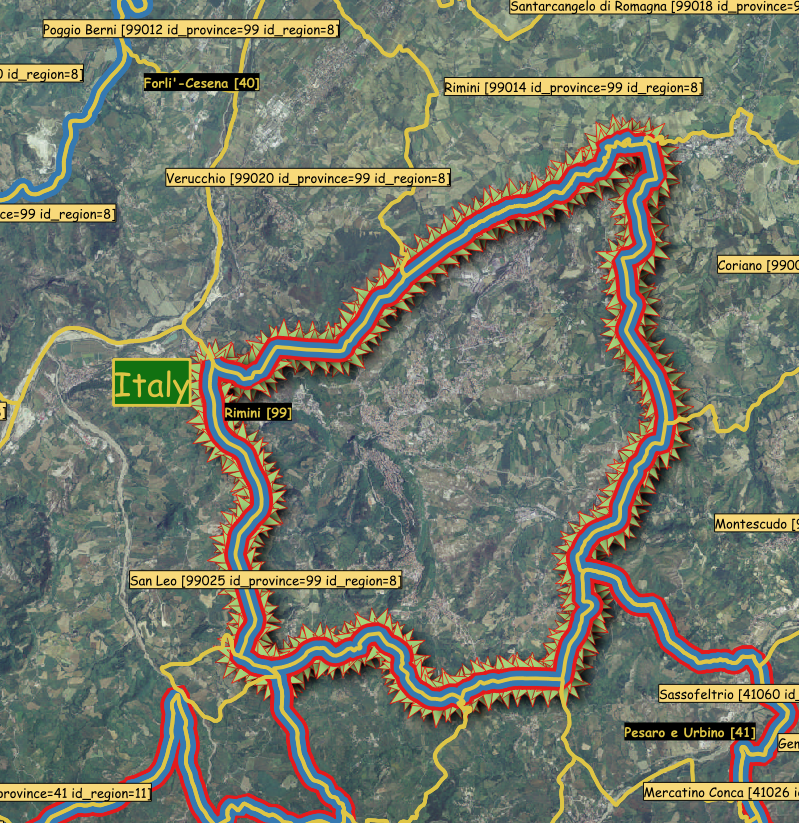
Explanation of Image: Area San Marino

• The Community boundries (yellow) id_city IN (41033,41035,41060,99003,99010,99014,99020,99025)
• The Province boundries (blue) id_province IN (41,99)
• The Region boundries (red) id_region IN (8,11)
• The Country boundries (green stars) id_country IN (39)

---

A Sql-Query to analyse the geometrys and work out the information needed later for the INSERT command.

Notes:
  San Marino is not an enclave of any single Community, Province or Region.
    (it is an enclave of Italy, but not the only one)
  So a 'enclave' will be created by combining the neighboring Community geometries.
    and then extract the 'enclave' as done with the Vatican City.

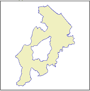
Communities:   1 POLYGON with 1 Interior-Ring	Provinces:   3 POLYGONs, 1 with 3 Interior-Rings
The Communities Geometry offers itself as the simplest solution

SELECT
 -- Communities: 1 Polygons, 1st with 1 Interior-Ring
 (SELECT ST_Union(geom_city) FROM admin_cities WHERE (id_city IN (41033,41035,41060,99003,99010,99014,99020,99025))) AS community_San_Marino,
 -- Provinces: 3 Polygons, 1st with 3 Interior-Ring
 (SELECT ST_Union(geom_province) FROM admin_provinces WHERE (id_province IN (41,99))) AS province_San_Marino,
 -- Regions: 4 Polygons, 2nd with 3 Interior-Ring (not shown as image)
 (SELECT ST_Union(geom_region) FROM admin_regions WHERE (id_region IN (8,11))) AS region_San_Marino,
 -- Select the first Interior-Ring of the first Polygon [1 based]
 (SELECT ST_InteriorRingN(ST_GeometryN(ST_Union(geom_city),1),1) FROM admin_cities WHERE (id_city IN (41033,41035,41060,99003,99010,99014,99020,99025))) AS linestring_San_Marino,
 -- Convert the Interior-Ring (closed LINESTRING) to a Polygon
 (SELECT ST_MakePolygon(ST_InteriorRingN(ST_GeometryN(ST_Union(geom_city),1),1)) FROM admin_cities WHERE (id_city IN (41033,41035,41060,99003,99010,99014,99020,99025))) AS polygon_San_Marino,
 -- Convert the Polygon to a MULTIPOLYGON for the admin_regions TABLE
 (
  -- -start- of sub-query
  SELECT
   -- create a MULTIPOLYGON from a POLYGON
   CastToMulti
   (
    -- create a POLYGON from a closed LINESTRING, non-aggregate-geometry input
    ST_MakePolygon
    (
     -- Interior-Ring (closed LINESTRING), non-aggregate-geometry input
     ST_InteriorRingN
     (
      -- which Interior-Ring number, 1-based
      ST_GeometryN
      (
       -- non-aggregate-geometry input
       ST_Union
       (
        -- aggregate-geometry input
        geom_city
       ),
       -- which geometry from collection, 1-based
       1
      ),
     -- which Interior-Ring number, 1-based
     1
    )
   )
  )
  FROM admin_cities
  WHERE
  (
   -- condition for aggregate-geometry input
   (id_city IN (41033,41035,41060,99003,99010,99014,99020,99025))
  )
  -- -end- of sub-query
 ) AS multi_polygon_San_Marino;

Conclusions:

• using community_San_Marino is simpler to use than the Province and Regions versions
• the POLYGON extraction is almost the same as the used for the Vatican City.
   The aggregate function ST_Union is used to create the geometry that the non-aggregate function ST_GeometryN needs.
  
• more details about this Sql-Query can be found in the Sql-HowTo

Here, again, you see that the combination of different Spatial-Functions gives you different results.

---

INSERT Sql: San Marino

INSERT INTO admin_regions
(id_region, name_region, population_region, area_region, city_count, province_count, id_country, name_country, geom_region)
 SELECT
  -- County calling (telephon) code
  378 AS id_region,
  'Repubblica di San Marino (Serenissima Repubblica di San Marino)' AS name_region,
  -- Population of Region, as whole persons [wiki data]
  33537 AS population_region,
  -- Area of Region, in meters [61072552.870600 ; wiki: 612000]
  ST_Area(ST_MakePolygon(ST_InteriorRingN(ST_GeometryN(ST_Union(geom_city),1),1))) AS area_region,
  -- Amount of Cities belonging to the Region,
  9 AS city_count,
  -- Amount of Provinces belonging to the Region,
  0 AS province_count,
  -- override default values for id_country and name_country
  378 AS id_country,
  'Republic of San Marino' AS name_country,
  -- Extract from Community of Rome geometry and stored as MULTIPOLYGON
  CastToMulti(ST_MakePolygon(ST_InteriorRingN(ST_GeometryN(ST_Union(geom_city),1),1))) AS geom_region
 FROM admin_cities
 WHERE
 (
  (id_city IN (41033,41035,41060,99003,99010,99014,99020,99025))
 );

---

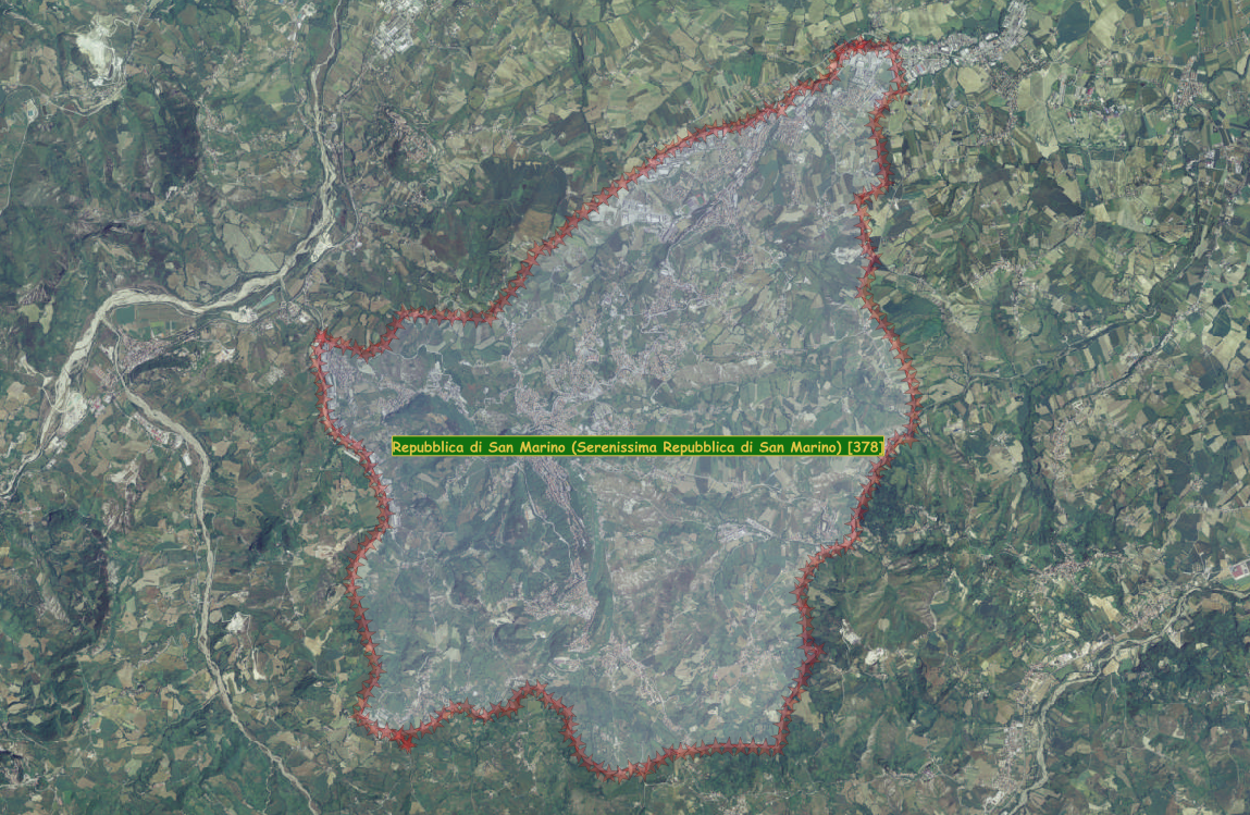
Then you can display the admin_regions, with filter id_region=378, in QGIS.

And now we present, (... da,da,da,daaa ...)
  the oldest, serviving, constitutional republic and the the fifth smallest country in the world:

Creation of the TABLE admin_countries

As a final step you can now create the admin_countries table representing the whole Italian Republic international boundaries.

-- this can take some time [ST_Area, ST_Union etc.], start TRANSACTION
BEGIN;
-- not being the first version of our masterpiece, remove previous version
DROP TABLE IF EXISTS admin_countries;

---

CREATE TABLE admin_countries
(
 -- based on County calling (telephon) code
 id_country INTEGER NOT NULL PRIMARY KEY,
 name_country TEXT NOT NULL,
 -- Population of Region, as whole persons
 population_country INTEGER DEFAULT 0,
 -- Area of Country, in meters
 area_country DOUBLE DEFAULT 0,
 -- Amount of Cities belonging to the Country,
 city_count INTEGER DEFAULT 0,
 -- Amount of Provinces belonging to the Country,
 province_count INTEGER DEFAULT 0,
 -- Amount of Regions belonging to the Country,
 region_count INTEGER DEFAULT 0
);

---

SELECT
 AddGeometryColumn('admin_countries', 'geom_country', 32632, 'MULTIPOLYGON', 'XY');
SELECT
 CreateSpatialIndex('admin_countries','geom_country');

---

-- This geometry is only needed for tutorial purposes, not needed for a real life scenario
SELECT
 AddGeometryColumn('admin_countries', 'bbox_geom_country', 32632, 'MULTIPOLYGON', 'XY');
SELECT
 CreateSpatialIndex('admin_countries','bbox_geom_country');

---

INSERT INTO admin_countries
(id_country, name_country, population_country, area_country, city_count, province_count, region_count, geom_country)
SELECT
 id_country,
 name_country,
 -- Population of Country, as whole persons
 sum(population_region) AS population_country,
 -- Area of Country, in meters
 ST_Area(ST_Union(geom_region)) AS area_country,
 -- Amount of Cities belonging to the Country,
 sum(city_count) AS city_count,
 -- Amount of Provinces belonging to the Country
 sum(province_count) AS province_count,
 -- Amount of Provinces belonging to the Country
 count(id_region) AS region_count,
 -- Build outer Boundry of the Country, based on Region-Geometries and stored as MULTIPOLYGON
 CastToMultiPolygon(ST_Union(geom_region)) AS geom_country
FROM admin_regions
-- for each UNIQUE id_country in admin_regions, create and INSERT into admin_countries.
GROUP BY id_country;

After the admin_countries has been filled, the not so stricly needed, bbox_geom_country can be created.

Preconditions for this to work correctly is:

• that the CreateSpatialIndex for geom_country command was executed

-- Such a geometry is only needed for tutorial purposes.
UPDATE admin_countries SET bbox_geom_country =
(
 SELECT
  CastToMultiPolygon
  (
   -- shows Bounding Box as Exterior-Ring, geometry as Interior-Ring
   ST_Difference
   (
    -- SpatialIndex of geometry of the boundries of the country
    BuildMbr
    (
     idx_SpatialIndex.xmin,
     idx_SpatialIndex.ymax,
     idx_SpatialIndex.xmax,
     idx_SpatialIndex.ymin,
     32632
    ),
    -- geometry of the boundries of the country
    geom_country
   )
  )
 FROM idx_admin_countries_geom_country AS idx_SpatialIndex
 WHERE
 (
  (idx_SpatialIndex.pkid=admin_countries.id_country)
 )
);

more details about this Sql-Query can be found in the Sql-HowTo

-- end TRANSACTION
COMMIT;

---

Then you can display the admin_countries     Shown here with the BoundingBox of the SpatialIndex around Italy, against Map of Ancient Italy around 49 BC.