Note:
The TABLEs created will be used in later recipes: (recipe #11, 12, 13, 14)
Normal Form
Editoral comment:
Italian National (ISTAT) Census 2011
The original dataset used in 'Cookbook 3.0' used SRID: 23032 - ED50 / UTM zone 32N
The present dataset used in 'Cookbook 5.0' uses SRID: 32632 - WGS 84 / UTM zone 32N
Many of the original images used here still show 23032 instead of 32632.
The TABLE and Columm names have been adapted to the present dataset.
Any
well designed DB adheres to the
relational paradigm, and implements the so-called
Normal Form.
Very simply explained in plain words:
- you'll first attempt to identify any distinct category (aka class) present into your dataset
- and simultaneously you have to identify any possible relation connecting categories.
- data redundancy is strongly discouraged, and has to be reduced whenever is possible.
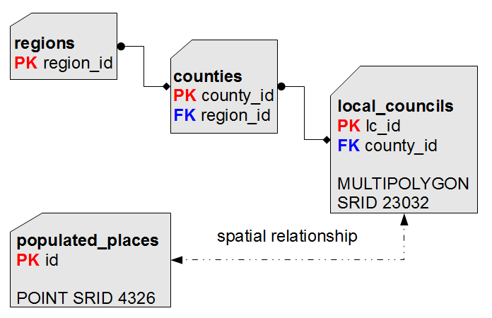
Consider the
ISTAT Census 2011; identifying categories and relations is absolutely simple:
- At the lowermost hierarchy level we have obviously Communities.
- Each Local Council surely belongs to some County: so a relation exists connecting Communities and Provinces.
To be more descriptive, this one is a typical one-to-many relationship
(one single County / many Communities: placing the same Local Council on two different Provinces is absolutely forbidden).
- The same is true for Provinces and Regions.
- There is not real need to establish a relation between Communities and Regions, because we can get this relation using the County as an intermediate pivot.
Accordingly to this, it's quite easy to identify several flaws in the original
Shapefile's layout:
- a pop_2011. value is present for Communities, Provinces and Regions:
well, this one clearly is an unneeded redundancy.
We simply have to preserve this information at the lowermost level (Communities):
because we can then compute anyway an aggregate value for Provinces (or Regions).
- a second redundancy exists: there is no real need compelling us to store both County and Region codes for each Local Council.
Preserving the County code is just enough, because we can get a reference to the corresponding Region anyway simply referencing the County.
- a Geometry representation is stored for each County and Region:
this too represents an unneeded redundancy, because we can get such Geometries simply aggregating the ones stored at the Local Council level.
Then we have the
cities1000. dataset: which comes from a completely different source (so there is no useful key we can use to establish relations to other entities).
And this dataset is in the
4326 SRID. (
WGS84), whilst any
ISTAT - Census 2011 dataset is in the
32632 SRID. [
WGS 84 / UTM zone 32N];
so for now will simply keep this dataset in a completely self-standing state.
We'll see later how we can actually integrate this dataset with the other ones: after all, all them represent Italy, isn't ?
For sure some geographic relationship must exist ...
 |
images need to be updated
- from SRID 4326 and 23032 to SRID 32632
|
Step 1a) we'll start by creating the
regions. table (i.e. hierarchical level 1).
CREATE TABLE regions
(
region_id INTEGER NOT NULL PRIMARY KEY,
region_name TEXT NOT NULL
);
Please note: we have defined a
PRIMARY KEY, i.e. a unique (not duplicable), absolutely unambiguous identifier for each Region.
Step 1b) then we'll populate the
regions. table.
INSERT INTO regions
(region_id, region_name)
SELECT
cod_reg AS region_id,
regione AS region_name
FROM reg2011_s
ORDER BY region_name;
Using the
INSERT INTO ... SELECT ... is more or less like performing a copy:
rows are extracted from the input table and immediately inserted into the output table.
As you can see, corresponding columns are explicitly identified
by order.
Step 2a) Now the same for
provinces, first
creating (i.e. hierarchical level 2). ....
CREATE TABLE provinces
(
province_id INTEGER NOT NULL PRIMARY KEY,
province_name TEXT NOT NULL,
car_plate_code TEXT NOT NULL,
region_id INTEGER NOT NULL,
CONSTRAINT fk_province_region
FOREIGN KEY (region_id)
REFERENCES regions (region_id)
);
... then
filling....
INSERT INTO provinces
(province_id, province_name,car_plate_code, region_id)
SELECT
cod_pro AS province_id,
provincia AS province_name,
sigla AS car_plate_code,
cod_reg AS region_id
FROM prov2011_s
ORDER BY province_name;
Note: Due to the defined CONSTRAINT
this command would fail if regions had not been filled beforhand.
Step 2b) create an
INDEX for the
relation between the
province and
region tables.
Please note: The relation exists through the definition of the
FOREIGN KEY..
CREATE INDEX idx_province_region ON provinces (region_id);
Short explanation:
An
index is used to support a
fast direct access to each single row.
- for a PRIMARY KEY, this is done automaticly in SQLite
- for a FOREIGN KEY, this is not done automaticly
What is the
default use of a
FOREIGN KEY, you may ask ...
It is a form of constraint, preventing a record to be INSERTed, when a condition is not fulfilled .
Sample: The Province of Firenze.in the Region of Toscana, cannot be INSERTed if the Region of Toscana does not exist.
So when a
fast direct access for a
FOREIGN KEY is needed
You must create and index from the FOREIGN KEY in the source TABLE (provinces), which reflect the values of the PRIMARY KEY of the referenced TABLE (regions) .
Step 3a) we'll now create the
communities. table (i.e. hierarchical level 3).
CREATE TABLE communities
(
community_id INTEGER NOT NULL PRIMARY KEY,
community_name TEXT NOT NULL,
population INTEGER NOT NULL,
province_id INTEGER NOT NULL,
CONSTRAINT fk_community_province
FOREIGN KEY (province_id)
REFERENCES provinces (province_id)
);
Since this will be used often to
retrive the province name from the the referenced TABLE
this must be fast, so we will create an INDEX.
CREATE INDEX idx_community_province ON communities (province_id);
Step 3b) creating a Geometry column for the
communities TABLE.
|
Placeholder: TODO: Proper explanadion of admin tasks for creation of geometry-column
Please note: we haven't defined any Geometry column, although one is required for communities.;
this is not a mistake, this is absolutely intentional. |
SELECT
AddGeometryColumn
(
-- the table-name
'communities',
-- the geometry column-name
'geometry',
-- the SRID to be used
32632,
-- the geometry class
'MULTIPOLYGON',
-- the geometry dimension (simple 2D)
'XY'
);
-- Add support for SpatialIndex-Queries
SELECT
CreateSpatialIndex
(
-- the table-name
'communities',
-- the geometry column-name
'geometry'
);
Step 3b) creating a Geometry column isn't the same as creating any other ordinary column.
We have to use the
AddGeometryColumn() spatial function, specifying:
- the geometry column name
- the SRID to be used
- the expected geometry class
- the dimension model
(in this case, simple 2D)
INSERT INTO communities
(community_id,community_name, population, province_id, geometry)
SELECT
pro_com AS community_id,
comune AS community_name,
pop_2011 AS population,
cod_pro AS province_id,
geometry
FROM com2011_s
-- avoid empty names [1]
WHERE ( community_name <> '')
ORDER BY community_name;
Step 3c) after all this can populate the
communities. table as usual.
Step 4) you have now to perform the last step: creating (and populating) the
populated_places. table.
DROP TABLE IF EXISTS populated_places;
CREATE TABLE IF NOT EXISTS populated_places
(
id INTEGER NOT NULL PRIMARY KEY AUTOINCREMENT,
name TEXT NOT NULL,
-- latitude in decimal degrees (wgs84) [Y-Position]
latitude DOUBLE DEFAULT 0,
--longitude in decimal degrees (wgs84) [X-Position]
longitude DOUBLE DEFAULT 0
);
SELECT
AddGeometryColumn('populated_places', 'geometry',32632, 'POINT', 2);
-- Add support for SpatialIndex-Queries
SELECT
CreateSpatialIndex
(
-- the table-name
'populated_places',
-- the geometry column-name
'geometry'
);
INSERT INTO populated_places
(id,latitude, longitude,name, geometry)
SELECT
NULL,latitude, longitude, name, ST_Transform(MakePoint(longitude, latitude, 4326),32632)
FROM cities1000
WHERE
(country_code = 'IT');
|
Placeholder: TODO: Expand why lat/long to UTM zone 32N is being done here
Goals:
Avoid ST_Transform 'WSG84' to 'UTM zone 32N'
[ST_Transform(MakePoint(longitude, latitude, 4326),32632)]
Retain lat/log as extra columns
Explain when:
An imported geometry in one SRID should be permanently / one-time or temporarily / on-the-fly Transformed.
- When the same data is often / always being transformed:
permanently / one-time should be done
- When the same data is seldom / one a year:
temporarily / on-the-fly should be done
|
Several interesting points to be noted:
- we have used an AUTOINCREMENT. clause for the PRIMARY KEY
- this practically means that SQLite can automatically generate an appropriate unique value for this PRIMARY KEY, when no explicit value has been already set.
- accordingly to this, in the INSERT INTO. statement a NULL. value was set for the PRIMARY KEY:
and this explicitly solicited SQLite to assign automatic values.
- the original cities1000. dataset shipped two numeric columns for longitude [COL006.] and latitude [COL005.]:
so we have to use the MakePoint(). Spatial function in order to build a point-like Geometry.
- the original latitude/ longitude (SRID 4326) points will be transformed to SRID 32632. WGS 84 / UTM zone 32N [Geographic System] SRS to match the other geometries.
Just to recapitulate:
- You started this tutorial using Virtual Shapefiles (and Virtual CSV/TXT) tables.
- Such Virtual Tables aren't at all real DB tables: they aren't internally stored.
They simply are trivial external files accessed using an appropriate driver.
- Using Virtual Tables at first allowed you to test some simple and very basic SQL queries.
- But in order to test more complex SQL features any dataset have to be properly imported into the DBMS itself.
- And this step required creating (and then populating) internal tables, accordingly to a well designed layout.
DROP TABLE com2011_s;
DROP TABLE prov2011_s;
DROP TABLE reg2011_s;
DROP TABLE cities1000;
Step 5) and finally you can drop any
Virtual Table, because they aren't any longer useful.
Please note: dropping a
Virtual Shapefile or
Virtual CSV/TXT doesn't removes the corresponding
external data-source, but simply removes the connection with the current database.
You already know the basic foundations about simple SQL queries.
Any previous example encountered since now simply queried a single table:
anyway SQL has no imposed limits, so you can query an arbitrary number of tables at the same time.
But in order to do this you must understand how to correctly handle a JOIN..
SELECT
*
FROM provinces, regions;
| province_id |
province_name |
car_plate_code |
region_id |
region_id |
region_name |
| 1 |
Torino |
TO |
1 |
1 |
Piemonte |
| 1 |
Torino |
TO |
1 |
2 |
Valle d'Aosta/Vallée d'Aoste |
| 1 |
Torino |
TO |
1 |
3 |
Lombardia |
| 1 |
Torino |
TO |
1 |
4 |
Trentino-Alto Adige/Südtirol |
| 1 |
Torino |
TO |
1 |
5 |
Veneto |
| ... |
... |
... |
... |
... |
... |
Apparently this query immediately works;
but once you get a quick glance at the result-set you'll immediately discover something really puzzling:
- an unexpected huge number of rows has been returned.
- and each single Province seems to every possible Region.
Every time SQL queries two different tables at the same time, the
Cartesian Product of both datasets is calculated.
i.e. each row coming from the first dataset is
JOIN.ed with any possible row coming from the second dataset.
This one is a
blind combinatorial process, so it very difficultly can produce useful results.
And this process can easily generate a
really huge result-set: this must absolutely be avoided, because:
- a very long (very, very long) time may be required to complete the operation.
- you can easily exhaust operating system resources before completion.
All this said, it's quite obvious that some appropriate
JOIN condition has to be set in order to maintain under control the Cartesian Product, so to actually return only meaningful rows.
SELECT
*
FROM provinces, regions
WHERE
(provinces.region_id = regions.region_id);
This query is exactly the same of the previous one: but this time we introduced an appropriate
JOIN condition.
Some points to be noted:
- using two (or more) tables can easily lead to name ambiguity:
e.g. in this case we have two different columns named region_id., one in the provinces. table, the other in the regions. table.
- we must use fully qualified names to avoid any possible ambiguity:
e.g. provinces.region_id. identifies the region_id. column belonging to the provinces. table, in an absolutely unambiguous way.
- defining the WHERE provinces.region_id = regions.region_id. clause we impose an appropriate JOIN condition.
After this the Cartesian Product will be accordingly filtered, so to insert into the result-set only the rows actually satisfying the imposed condition, ignoring any other.
SELECT
p.province_id AS province_id,
p.province_name AS province_name,
p.car_plate_code AS car_plate_code,
r.region_id AS region_id,
r.region_name AS region_name
FROM provinces AS p,
regions AS r
WHERE
(p.region_id = r.region_id);
| province_id |
province_name |
car_plate_code |
region_id |
region_name |
| 1 |
Torino |
TO |
1 |
Piemonte |
| 2 |
Vercelli |
VC |
1 |
Piemonte |
| 3 |
Novara |
NO |
1 |
Piemonte |
| 4 |
Cuneo |
CN |
1 |
Piemonte |
| 5 |
Asti |
AT |
1 |
Piemonte |
| 6 |
Alessandria |
AL |
1 |
Piemonte |
| ... |
... |
... |
... |
... |
And this one always is the same as above, simply written adopting a most polite syntax:
- using extensively the AS. clause so to define alias names for both columns and tables make JOIN. queries to be much more concise and readable, and easiest to understand.
SELECT
c.community_id AS community_id,
c.community_name AS community_name,
c.population AS population,
p.province_id AS province_id,
p.province_name AS province_name,
p.car_plate_code AS car_plate_code,
r.region_id AS region_id,
r.region_name AS region_name
FROM communities AS c,
provinces AS p,
regions AS r
WHERE
(
(c.province_id = p.province_id) AND
(p.region_id = r.region_id)
);
| community_id |
community_name |
population |
province_id |
province_name |
car_plate_code |
region_id |
region_name |
| 1001 |
Agliè |
2574 |
1 |
Torino |
TO |
1 |
Piemonte |
| 1002 |
Airasca |
3554 |
1 |
Torino |
TO |
1 |
Piemonte |
| 1003 |
Ala di Stura |
479 |
1 |
Torino |
TO |
1 |
Piemonte |
| ... |
... |
... |
... |
... |
... |
... |
... |
Joining three (
or even more) tables isn't much more difficult:
you simply have to apply any required
JOIN condition as appropriate.
Performance considerations
Executing complex queries involving many different tables may easily run in a very slow and sluggish mode.
This will most easily noticed when such tables contain a huge number of rows.
Explaining all this isn't at all difficult: in order to calculate the Cartesian Product the SQL engine has to access many and many times each table involved in the query.
The basic behavior is the one to perform a
full table scan each time: and obviously scanning a long table many and many times requires a long time.
So the main key-point in order optimize your queries is the one to avoid using
full table scans as much as possible.
All this is fully supported, and it's easy to be implemented.
Each time the
SQL-planner (an internal component of the
SQL-engine) detects that an appropriate
INDEX. is available, there is no need at all to perform
full table scans, because each single row can now be immediately accessed using this Index.
And this one will obviously be a much faster process.
Any column (or group of columns) frequently used in
JOIN. clauses is a good candidate for a corresponding
INDEX..
Anyway, creating an Index implies several negative consequences:
- the storage allocation required by the DB-file will increase (sometimes will dramatically increase).
- performing INSERT., UPDATE. and/or DELETE. ops will require a longer time, because the Index has to be accordingly updated.
And this obviously imposes a further overhead.
So (not surprisingly) it's a
trade-off process: you must evaluate carefully when an
INDEX. is absolutely required, and attempt to reach a well balanced mix.
i.e a
compromise between contrasting requirements, under various conditions and in different users-cases.
In other words there is no
absolute rule: you must find your optimal
case-by-case solution performing several practical tests, until you get the optimal solution fulfilling your requirements.
SQL supports another alternative syntax to represent JOIN ops.
More or less both implementations are strictly equivalent, so using the one or the other simply is matter of personal taster in the majority of cases.
Anyway, this second method supports some really interesting further feature that is otherwise unavailable.
SELECT
c.community_id AS community_id,
c.community_name AS community_name,
c.population AS population,
p.province_id AS province_id,
p.province_name AS province_name,
p.car_plate_code AS car_plate_code,
r.region_id AS region_id,
r.region_name AS region_name
FROM communities AS c,
provinces AS p,
regions AS r
WHERE
(
(c.province_id = p.province_id) AND
(p.region_id = r.region_id)
);
You now feel a strong
deja vu sensation: and that's more than appropriate, because you have already encountered this query in the previous example.
SELECT
c.community_id AS community_id,
c.community_name AS community_name,
c.population AS population,
p.province_id AS province_id,
p.province_name AS province_name,
p.car_plate_code AS car_plate_code,
r.region_id AS region_id,
r.region_name AS region_name
FROM communities AS c
JOIN provinces AS p ON (c.province_id = p.province_id)
JOIN regions AS r ON (p.region_id = r.region_id);
All right, this one is the same identical query rewritten accordingly to alternative syntax rules:
- using the JOIN ... ON (...). clause makes more explicit what's going on.
- and JOIN. conditions are now directly expressed within the ON (...). term:
this way the query statement is better structured and more readable.
- anyway, all this simply is syntactic sugar:
there is no difference at all between the above two queries in functional terms.
SELECT
r.region_name AS region,
p.province_name AS province,
c.community_name AS community,
c.population AS population
FROM regions AS r
-- JOIN county to region, based on common .region_id
JOIN provinces AS p ON (p.region_id = r.region_id)
-- JOIN communities to county, based on common .province_id
-- - but only when communities > 100000
JOIN communities AS c ON ((p.province_id = c.province_id) AND (c.population > 100000))
ORDER BY r.region_name, province_name;
| region |
province |
community |
population |
| Abruzzo |
Pescara |
Pescara |
116286 |
| Calabria |
Reggio di Calabria |
Reggio di Calabria |
180353 |
| Campania |
Napoli |
Napoli |
1004500 |
| Campania |
Salerno |
Salerno |
138188 |
| Emilia-Romagna |
Bologna |
Bologna |
371217 |
| ... |
... |
... |
... |
There is nothing strange or new in this query:
- we simply introduced a further ON (... AND c.population < 100000). clause, so to exclude any small populated Local Council.
SELECT
r.region_name AS region,
p.province_name AS province,
c.community_name AS community,
c.population AS population
FROM regions AS r
JOIN provinces AS p ON (p.region_id = r.region_id)
LEFT JOIN communities AS c ON ((p.province_id = c.province_id) AND (c.population > 100000))
ORDER BY r.region_name, province_name;
| region |
province |
community |
population |
| Abruzzo |
Chieti |
NULL |
NULL |
| Abruzzo |
L'Aquila |
NULL |
NULL |
| Abruzzo |
Pescara |
Pescara |
116286 |
| Abruzzo |
Teramo |
NULL |
NULL |
| Basilicata |
Matera |
NULL |
NULL |
| Basilicata |
Potenza |
NULL |
NULL |
| ... |
... |
... |
... |
Apparently this query is the same as the latest one.
But a remarkable difference exists:
- this time we've used a LEFT JOIN. clause:
and the result-set now looks very different from the previous one.
- a plain JOIN. clause will include into the result-set only rows for which both the left-sided and the right-sided terms has been positively resolved.
- but the most sophisticated LEFT JOIN. clause will include into the result-set any row having an unresolved right-sided term:
and in this case any right-sided member assumes a NULL. value.
There is a striking difference between a plain JOIN. and a LEFT JOIN..
Coming back to previous example, using a LEFT JOIN. clause ensures that any Region and any County will now be inserted into the result-set, even the ones failing to satisfy the imposed population limit for Communities.
SQL supports a really useful feature, the so called
VIEW.
Very shortly explained, a
VIEW is something falling half-way between a
TABLE. and a
query:
- a VIEW is a persistent objects (exactly as TABLE.s are).
- you can query a VIEW exactly in the same way you can query a TABLE.:
there is no difference at all distinguishing a VIEW and a TABLE. from the SELECT own perspective.
- but after all a VIEW simply is like a kind of glorified query.
A VIEW has absolutely no data by itself.
Data apparently belonging to some VIEW are simply retrieved from some other TABLE. each time they are actually required.
- in the SQLite's own implementation any VIEW strictly is a read-only object:
you can freely reference any VIEW in SELECT statements.
But attempting to perform an INSERT., UPDATE. or DELETE. statement on behalf of a VIEW isn't allowed.
Anyway, performing some practical exercise surely is the best way to introduce Views.
CREATE VIEW view_community AS
SELECT
c.community_id AS community_id,
c.community_name AS community_name,
c.population AS population,
p.province_id AS province_id,
p.province_name AS province_name,
p.car_plate_code AS car_plate_code,
r.region_id AS region_id,
r.region_name AS region_name,
c.geometry AS geometry
FROM communities AS c
JOIN provinces AS p ON (c.province_id = p.province_id)
JOIN regions AS r ON (p.region_id = r.region_id);
Et voila, here is your first
VIEW:
- basically, this looks exactly as any query you've already seen since now.
- except in this; this time the first line is: CREATE VIEW ... AS.
- and this one is unique syntactical difference transforming a plain query into a VIEW definition.
SELECT
community_name, population, province_name
FROM view_community
WHERE (region_name = 'Lazio')
ORDER BY community_name
| community_name |
population |
province_name |
| Accumoli |
724 |
Rieti |
| Acquafondata |
316 |
Frosinone |
| Acquapendente |
5788 |
Viterbo |
| Acuto |
1857 |
Frosinone |
| Affile |
1644 |
Roma |
| ... |
... |
... |
You can actually query this
VIEW.
SELECT
region_name,
Sum(population) AS population,
(Sum(ST_Area(geometry)) / 1000000.0) AS "area (sq.Km)",
(Sum(population) / (Sum(ST_Area(geometry)) / 1000000.0)) AS "popDensity (people/sq.Km)"
FROM view_community
GROUP BY region_id
-- '4'= 4th column (called 'popDensity (people/sq.Km)')
ORDER BY 4;
| region_name |
population |
area (sq.Km) |
popDensity (people/sq.Km) |
| Valle d'Aosta/Vallée d'Aoste |
119548 |
3258.405868 |
36.689107 |
| Basilicata |
597768 |
10070.896921 |
59.355984 |
| ... |
... |
... |
... |
| Marche |
1470581 |
9729.862860 |
151.140979 |
| Toscana |
3497806 |
22956.355019 |
152.367656 |
| ... |
... |
... |
... |
| Lombardia |
9032554 |
23866,529331 |
378.461144 |
| Campania |
5701931 |
13666.322146 |
417.224981 |
You can really perform any arbitrary complex query using a
VIEW.
SELECT
v.community_name AS Community,
v.province_name AS Province,
v.region_name AS Region
FROM view_community AS v
JOIN communities AS c ON
(
-- with: (Upper(c.community_name) = 'NORCIA') : 4 min 22.883 seconds ; without 1.427 seconds
(c.community_name = 'Norcia') AND
(ST_Touches(v.geometry, c.geometry))
)
ORDER BY v.community_name, v.province_name, v.region_name;
| Community |
Province |
Region |
| Accumoli |
Rieti |
Lazio |
| Arquata del Tronto |
Ascoli Piceno |
Marche |
| Cascia |
Perugia |
Umbria |
| Castelsantangelo sul Nera |
Macerata |
Marche |
| Cerreto di Spoleto |
Perugia |
Umbria |
| Cittareale |
Rieti |
Lazio |
| Montemonaco |
Ascoli Piceno |
Marche |
| Preci |
Perugia |
Umbria |
You can
JOIN. a
VIEW and a
TABLE. (or two
VIEWs, and so on ...)
Just a simple explanation: this
JOIN. actually is one based on Spatial relationships:
the result-set represents the list of Communities sharing a common boundary with the
Norcia one.
You can get a much more complete example
here (
Haute cuisine recipes).
A VIEW is one of the many powerful and wonderful features supported by SQL.
And SQLite's own implementation for VIEW surely is a first class one.
You should use VIEW as often as you can: and you'll soon discover that following this way handling really complex DB layouts will become a piece of cake.
Please note: querying a VIEW can actually be as fast and efficient as querying a TABLE..
But a VIEW cannot anyway be more efficient than the underlying query is; any poorly designed and badly optimized query surely will translate into a very slow VIEW.
You are now well conscious that SQL overall performance and efficiency strongly depend on the underlying
database layout, i.e. the following design choices are critical:
- defining tables (and columns) in the most appropriate way.
- identifying relations connection different tables.
- supporting often-used relations with an appropriate index.
- identifying useful constraints, so to preserve data consistency and correctness as much as possible.
It's now time to examine in deeper detail such topics.
Pedantic note: in
DBMS/SQL. own jargon all this is collectively defined as
DDL. [
Data Definition Language], and is intended as opposed to
DML. [
Data Manipulation Language], i.e.
SELECT,
INSERT. and so on.
CREATE TABLE people
(
first_name TEXT,
last_name TEXT,
age INTEGER,
gender TEXT,
phone TEXT
);
This statement will create a very simple
table named
people.:
- each individual column definition must at least specify the corresponding data-type, such as TEXT. or INTEGER.
- please note: data-type handling in SQLite strongly differs from others DMBS implementations:
but we'll see this in more detail later.
CREATE TABLE people2
(
id INTEGER NOT NULL PRIMARY KEY AUTOINCREMENT,
first_name TEXT NOT NULL,
last_name TEXT NOT NULL,
age INTEGER CONSTRAINT age_verify CHECK (age BETWEEN 18 AND 90),
gender TEXT CONSTRAINT gender_verify CHECK (gender IN ('M', 'F')),
phone TEXT
);
This one is more sophisticated version of the same table:
- we have added an id. column, declared as PRIMARY KEY AUTOINCREMENT.
- inserting a PRIMARY KEY on each table always is a very good idea.
- declaring an AUTOINCREMENT. clause we'll request SQLite to automatically generate unique values for this key.
- we have added a NOT NULL. clause for first_name. and last_name. columns.
- this will declare a first kind of constraint: NULL. values will be rejected for these columns.
- in other words, first_name. and last_name. absolutely have to contain some explicitly set value.
- we have added a CONSTRAINT ... CHECK (...). for age. and gender. columns.
- this will declare a second kind of constraint: values failing to satisfy the CHECK (...). criterion will be rejected.
- the age. column will now accept only reasonable adult ages.
- and the gender. column will now accept only 'M'. or 'F'. values.
- please note: we have not declared the NOT NULL. clause, so age = NULL. and gender = NULL. are still considered to be valid values.
about SQLite data-types
Very shortly said: SQLite hasn't data-types at all ...
You are absolutely free to insert any data-type on every column: the column declared data-type simply have a
decorative role, but isn't neither checked not enforced at all.
This one absolutely is not a
bug: it's more a
peculiar design choice.
Anyway, any other different DBMS applies strong data-type qualification and enforcement, so the SQLite's own behavior may easily look odd and puzzling.
Be warned.
Anyway SQLite internally supports the following data-types:
- NULL.: no value at all.
- INTEGER.: actually 64bit integers, so to support really huge values.
- DOUBLE.: floating point, double precision.
- TEXT.: any UTF-8 encoded text string, of unconstrained arbitrary length.
- BLOB.: any generic Binary Long Object, of unconstrained arbitrary length.
Remember: each single
cell (
row/column intersection) can store any arbitrary data-type.
One unique exception exists: columns declared as
INTEGER PRIMARY KEY. absolutely require integer values.
You can
add any further column after the initial table creation with ...
ALTER TABLE people2
ADD COLUMN cell_phone TEXT;
Yet another SQLite's own very
peculiar design choice.
- dropping columns is unsupported.
- renaming columns is unsupported.
i.e. once you've created a column there is no way at all to change its initial definition.
[
2018-09-15] Starting with
SQLite 3.25 :
- Add support for renaming columns within a table using ALTER TABLE table RENAME COLUMN oldname TO newname.
- Fix table rename feature so that it also updates references to the renamed table in triggers and views.
You can
change the table name with ...
ALTER TABLE people2
RENAME TO people_ok;
Or
remove the table (and its whole content) from the Database with ...
DROP TABLE people;
You can
create an Index with ...
CREATE INDEX idx_people_phone ON people_ok (phone);
Or
destroy a Index with ...
DROP INDEX idx_people_phone;
To
create an Index that support more than one column with ...
CREATE UNIQUE INDEX idx_people_name ON people_ok (last_name, first_name);
- declaring the UNIQUE. clause implements a further constraint:
once some value is already defined, any further attempt to insert the same value will then fail.
In order to query a
table layout you can use
PRAGMA table_info(people_ok);
| cid |
name |
type |
notnull |
dflt_value |
pk |
| 0 |
id |
INTEGER |
1 |
NULL |
1 |
| 1 |
first_name |
TEXT |
1 |
NULL |
0 |
| 2 |
last_name |
TEXT |
1 |
NULL |
0 |
| 3 |
age |
INTEGER |
0 |
NULL |
0 |
| 4 |
gender |
TEXT |
0 |
NULL |
0 |
| 5 |
phone |
TEXT |
0 |
NULL |
0 |
| 6 |
cell_phone |
TEXT |
0 |
NULL |
0 |
You can easily query the corresponding Index layout by
using
PRAGMA index_list(people_ok);
| seq |
name |
unique |
| 0 |
idx_people_phone |
0 |
| 1 |
idx_people_name |
1 |
and
PRAGMA index_info(idx_people_name);
| seqno |
cid |
name |
| 0 |
2 |
last_name |
| 1 |
1 |
first_name |
We'll now examine in deeper detail how to correctly define a Geometry-type column.
SpatiaLite follows an approach very closely related to the one adopted by PostgreSQL/PostGIS;
i.e. creating a Geometry-type at the same time the corresponding table is created isn't allowed.
You must first
create the table, with the '
normal'-columns ...
CREATE TABLE cities_test
(
id_geoname INTEGER NOT NULL PRIMARY KEY AUTOINCREMENT,
name TEXT DEFAULT '',
-- Y-Position,
latitude DOUBLE DEFAULT 0,
-- X-Position,
longitude DOUBLE DEFAULT 0
);
Then
add the Geometry-column, as a separate step ...
SELECT
AddGeometryColumn('cities_test', 'geom_wsg84',4326, 'POINT', 'XY');
This is the
proper way to insure that a completely valid / usable Geometry-colulmn will be created.
Any different approach will lead incorrect and unreliable Geometry.
Although the previous command more commonly used, another form, supported by
AddGeometryColumn(), exists:
SELECT AddGeometryColumn
(
-- table-name
'cities_test',
-- geometry column-name
'geom_wsg84',
-- srid of geometry
4326,
-- geometry-type
'POINT',
-- permit NULL values for geometry [0=yes ; 1=no]
0
);
The last (
optional) argument actually means:
NOT NULL.
- setting a value 0. (the default value, if omitted) then the Geometry column will accept NULL. values.
- otherwise only NOT NULL. geometries will be accepted.
Supported
SRIDs:
- any possible SRID defined within the spatial_ref_sys. metadata table.
including the 2 Undefined shown below
The standard
OGC-SFS defines 2 forms of an
Undefined SRIDs:
-
-1: 'Undefined - Cartesian' [default]
- pixels: of non-georeferenced images
- unknown: with values that are not in degrees
-
0: 'Undefined - Geographic Long/Lat'
- old maps: with no projection information, but using degrees
-
unknown: but with degrees values
Y/latitude (+90 to -90) or X/longitude (+180 to -180)
In most cases
Spatialite assumes
-1: 'Undefined - Cartesian'
when a SRID is not defined.
Supported
Geometry-types:
| POINT |
The commonly used Geometry-types:
corresponding to Shapefile's specs and supported by any desktop GIS apps
|
| LINESTRING |
| POLYGON |
| MULTIPOINT |
| MULTILINESTRING |
| MULTIPOLYGON |
| GEOMETRYCOLLECTION |
Not often used: unsupported by Shapefile and desktop GIS apps |
| GEOMETRY |
A generic container supporting any possible geometry-class
Not often used: unsupported by Shapefile and desktop GIS apps |
Supported
Dimension-models:
| XY |
2 |
X and Y coords (simple 2D) |
| XYZ |
3 |
X, Y and Z coords (3D) |
| XYM |
-
|
X and Y coords + measure value M |
| XYZM |
4
|
X, Y and Z coords + measure value M |
Please note well: this one is a very frequent pitfall.
Many developers, GIS professionals and alike obviously feel to be much smarter than this, so they often tend to invent some highly imaginative alternative way to create their own Geometries.
e.g. bungling someway the geometry_columns table seems to be a very popular practice.
May well be that such creative methods will actually work with some very specific SpatiaLite's version; but for sure some severe incompatibility will raise before or after ...
Be warned: only Geometries created using AddGeometryColumn() are fully legitimate.
Any different approach is completely unsafe (and unsupported ..)
I suppose that directly checking how AddGeometryColumn() affects the database may help you to understand better.
PRAGMA table_info(cities_test);
| cid |
name |
type |
notnull |
dflt_value |
pk |
| 0 |
id |
INTEGER |
1 |
NULL |
1 |
| 1 |
name |
TEXT |
1 |
'' |
0 |
| 2 |
latitude |
DOUBLE |
1 |
0 |
0 |
| 2 |
longitude |
DOUBLE |
1 |
0 |
0 |
| 3 |
geom_wsg84 |
POINT |
0 |
NULL |
0 |
step 1: a new
geom_wsg84. column has been added to the corresponding table.
SELECT
*
FROM geometry_columns
WHERE
(f_table_name LIKE 'cities_test');
| f_table_name |
f_geometry_column |
geometry_type |
coord_dimension |
srid |
spatial_index_enabled |
| cities_test |
geom_wsg84 |
1 |
2 |
4326 |
0 |
step 2: a corresponding row has been inserted into the
geometry_columns metadata table.
SELECT
*
FROM sqlite_master
WHERE
(
(type = 'trigger') AND
(tbl_name LIKE 'cities_test')
);
| type |
name |
tbl_name |
rootpage |
sql |
| trigger |
ggi_cities_test_geom_wsg84 |
cities_test |
0 |
CREATE TRIGGER "ggi_cities_test_geom_wsg84" BEFORE INSERT ON "cities_test"
FOR EACH ROW BEGIN
SELECT RAISE(ROLLBACK, 'cities_test.geom_wsg84 violates Geometry constraint [geom-type or SRID not allowed]')
WHERE (SELECT geometry_type FROM geometry_columns
WHERE Lower(f_table_name) = Lower('cities_test') AND Lower(f_geometry_column) = Lower('geom_wsg84')
AND GeometryConstraints(NEW."geom_wsg84", geometry_type, srid) = 1) IS NULL;
END |
| trigger |
ggu_cities_test_geom_wsg84 |
cities_test |
0 |
CREATE TRIGGER "ggu_cities_test_geom_wsg84" BEFORE UPDATE OF "geom_wsg84" ON "cities_test"
FOR EACH ROW BEGIN
SELECT RAISE(ROLLBACK, 'cities_test.geom_wsg84 violates Geometry constraint [geom-type or SRID not allowed]')
WHERE (SELECT geometry_type FROM geometry_columns
WHERE Lower(f_table_name) = Lower('cities_test') AND Lower(f_geometry_column) = Lower('geom_wsg84')
AND GeometryConstraints(NEW."geom_wsg84", geometry_type, srid) = 1) IS NULL;
END |
| trigger |
tmu_cities_test_geom_wsg84 |
cities_test |
0 |
CREATE TRIGGER "tmu_cities_test_geom_wsg84" AFTER UPDATE ON "cities_test"
FOR EACH ROW BEGIN
UPDATE geometry_columns_time SET last_update = strftime('%Y-%m-%dT%H:%M:%fZ', 'now')
WHERE Lower(f_table_name) = Lower('cities_test') AND Lower(f_geometry_column) = Lower('geom_wsg84');
END |
| trigger |
tmi_cities_test_geom_wsg84 |
cities_test |
0 |
CREATE TRIGGER "tmi_cities_test_geom_wsg84" AFTER INSERT ON "cities_test"
FOR EACH ROW BEGIN
UPDATE geometry_columns_time SET last_insert = strftime('%Y-%m-%dT%H:%M:%fZ', 'now')
WHERE Lower(f_table_name) = Lower('cities_test') AND Lower(f_geometry_column) = Lower('geom_wsg84');
END |
| trigger |
tmd_cities_test_geom_wsg84 |
cities_test |
0 |
CREATE TRIGGER "tmd_cities_test_geom_wsg84" AFTER DELETE ON "cities_test"
FOR EACH ROW BEGIN
UPDATE geometry_columns_time SET last_delete = strftime('%Y-%m-%dT%H:%M:%fZ', 'now')
WHERE Lower(f_table_name) = Lower('cities_test') AND Lower(f_geometry_column) = Lower('geom_wsg84');
END |
step 3: the
sqlite_master. is the main
metadata table used by SQLite to store internal objects.
As you can easily notice, each Geometry requires some
triggers to be fully supported and well integrated into the DBMS workflow.
Not at all surprisingly, all this has to be defined in a strongly self-consistent way in order to let SpatiaLite work as expected.
If some element is missing or badly defined, the obvious consequence will be a defective and unreliable Spatial DBMS.
SELECT
DiscardGeometryColumn('cities_test', 'geom_wsg84');
This will remove any
metadata and any
trigger related to the given Geometry.
Please note: anyway this will leave any geometry-value stored within the corresponding table absolutely untouched.
Simply, after calling
DiscardGeometryColumn(...). they aren't any longer fully qualified geometries, but anonymous and generic BLOB values.
SELECT
RecoverGeometryColumn('cities_test', 'geom_wsg84',4326, 'POINT', 2);
This will attempt to recreate any
metadata and any
trigger related to the given Geometry.
If the operation successfully completes, then the Geometry column is fully qualified.
In other words, there is absolutely no difference between a Geometry created by
AddGeometryColumn() and another created by
RecoverGeometryColumn().
Very simply explained:
- AddGeometryColumn() is intended to create a new, empty column.
- RecoverGeometryColumn() is intended to recover in a second time an already existing (and populated) column.
Sometimes circumventing version-related issues is inherently impossible: e.g. there is absolutely no way to use 3D geometries on obsolescent versions, because the required support was introduced in more recent times.
But in many other cases such issues are simply caused by some incompatible binary function required by
triggers.
Useful hint
To resolve any trigger-related incompatibility you can simply try to:
- remove first any trigger: the best way you can follow is using DiscardGeometryColumn().
- and then recreate again the triggers using AddGeometryColumn()
This will ensure that any
metadata info and
trigger will surely match expectations of your binary library current version.
Since now we've mainly examined how to query tables.
SQL isn't obviously a read-only language: inserting new rows, deleting existing rows and updating values is supported in the most flexible way.
It's now time to examine such topics in deeper detail.
CREATE TABLE cities_test
(
id_geoname INTEGER NOT NULL PRIMARY KEY AUTOINCREMENT,
name TEXT DEFAULT '',
-- Y-Position,
latitude DOUBLE DEFAULT 0,
-- X-Position,
longitude DOUBLE DEFAULT 0
);
SELECT
AddGeometryColumn('cities_test', 'geom_wsg84', 4326, 'POINT', 'XY');
Nothing new in this: it's exactly the same table we've already created in the previous example.
INSERT INTO cities_test
(id_geoname, name, latitude, longitude, geom_wsg84)
VALUES(NULL, 'first point', 1.02, 1.01, GeomFromText('POINT(1.01 1.02)', 4326));
INSERT INTO cities_test
VALUES(NULL, 'second point', 2.02, 2.01,GeomFromText('POINT(2.01 2.02)', 4326));
INSERT INTO cities_test
(id_geoname, name, latitude, longitude, geom_wsg84)
VALUES(10, 'tenth point', 10.02, 10.01,GeomFromText ('POINT(10.01 10.02)', 4326));
INSERT INTO cities_test
(geom_wsg84, latitude, longitude, name, id_geoname)
VALUES(GeomFromText('POINT(11.01 11.02)', 4326), 11.02, 11.01, 'eleventh point', NULL);
INSERT INTO cities_test
(id_geoname, latitude, longitude, geom_wsg84, name)
VALUES(NULL, 12.02, 12.01, NULL, 'twelfth point');
The
INSERT INTO (...) VALUES (...). statement does exactly what its name states:
- the first list enumerates the column names
- and the second list contains the values to be inserted: correspondences between columns and values are established by position.
- you can simply suppress the column-names list (please, see the second INSERT. statement):
anyway this one isn't a good practice, because such statement implicitly relies upon some default column order, and that's not at all a safe assumption.
- another interesting point; this table declares a PRIMARY KEY AUTOINCREMENT.:
- as a general rule we've passed a corresponding NULL. value, so to allow SQLite autogenerating a unique value.
- but in the third INSERT. we've set an explicit value (please, check in the following paragraph what really happens in this case).
SELECT
*
FROM cities_test;
| id_geoname |
name |
latitude |
longitude |
geom_wsg84 |
| 1 |
first point |
1.02 |
1.01 |
BLOB sz=60 GEOMETRY |
| 2 |
second point |
2.02 |
2.01 |
BLOB sz=60 GEOMETRY |
| 10 |
tenth point |
10.02 |
10.01 |
BLOB sz=60 GEOMETRY |
| 11 |
eleventh point |
11.02 |
11.01 |
BLOB sz=60 GEOMETRY |
| 12 |
twelfth point |
12.02 |
12.01 |
NULL |
Just a quick check before going further on ...
INSERT INTO cities_test
VALUES(2, 'POINT #2', 2.02, 2.01, GeomFromText('POINT(2.01 2.02)', 4326));
This further
INSERT. will
loudly fail, raising a
constraint failed exception.
Accounting for this isn't too much difficult: a
PRIMARY KEY always enforces a
uniqueness constraint.
And actually one row of
id = 2 already exists into this table.
INSERT OR IGNORE INTO cities_test
VALUES(2, 'POINT #2', 2.02, 2.01,,GeomFromText('POINT(2.01 2.02)', 4326));
By specifying an
OR IGNORE. clause this statement will now
silently fail (
same reason as before).
INSERT OR REPLACE INTO cities_test
VALUES(2, 'POINT #2', 2.02, 2.01,,GeomFromText('POINT(2.01 2.02)', 4326));
There is a further variant: i.e. specifying an
OR REPLACE. clause this statement will actually act like an
UPDATE.
REPLACE INTO cities_test
(id_geoname, name, latitude, longitude, geom_wsg84)
VALUES(3, 'POINT #3', 3.02, 3.01, GeomFromText('POINT(3.01 3.02)', 4326));
REPLACE INTO cities_test
(id_geoname, name, latitude, longitude, geom_wsg84)
VALUES(11, 'POINT #11', 11.32, 11.31,GeomFromText('POINT(11.31 11.32)', 4326));
And yet another syntactic alternative is supported, i.e. simply using
REPLACE INTO.:
but this latter simply is an
alias for
INSERT OR REPLACE..
SELECT
*
FROM cities_test;
| id_geoname |
name |
latitude |
longitude |
geom_wsg84 |
| 1 |
first point |
1.02 |
1.01 |
BLOB sz=60 GEOMETRY |
| 2 |
POINT #2 |
2.02 |
2.01 |
BLOB sz=60 GEOMETRY |
| 3 |
POINT #3 |
3.02 |
3.01 |
BLOB sz=60 GEOMETRY |
| 10 |
tenth point |
10.02 |
10.01 |
BLOB sz=60 GEOMETRY |
| 11 |
POINT #11 |
11.32 |
11.31 |
BLOB sz=60 GEOMETRY |
| 12 |
twelfth point |
12.02 |
12.01 |
NULL |
Just another quick check ...
UPDATE cities_test SET
name = 'point-3',
latitude = 3.320000,
longitude = 3.310000
WHERE (id_geoname = 3);
UPDATE cities_test SET
latitude = latitude + 45.0,
longitude = (longitude + 90.0)
WHERE (id_geoname > 10);
updating values isn't much more complex ...
DELETE FROM cities_test
WHERE ((id_geoname % 2) = 0);
and the same is for deleting rows.
i.e. this
DELETE. statement will affect every
even id value.
SELECT
*
FROM cities_test;
| id_geoname |
name |
latitude |
longitude |
geom_wsg84 |
| 1 |
first point |
1.02 |
1.01 |
BLOB sz=60 GEOMETRY |
| 3 |
point-3 |
3.320000 |
3.310000 |
BLOB sz=60 GEOMETRY |
| 11 |
POINT #11 |
56.320000 |
101.310000 |
BLOB sz=60 GEOMETRY |
A last final quick check ...
Very important notice
Be warned: calling an
UPDATE. or
DELETE. statement without specifying any corresponding
WHERE. clause is a full legal operation in SQL.
Anyway SQL intends that the corresponding change must indiscriminately affect any row within the table: and sometimes this is exactly what you intended to do.
But (
much more often) this is a wonderful way allowing to
unintentionally destroy or to irreversibly corrupt your data:
beginner, pay careful attention.
Understanding what
constraints are is a very simple task following a
conceptual approach.
But on the other side understanding why some SQL statement will actually fail raising a generic
constraint failed exception isn't a so simple affair.
In order to let you understand better this paragraph is structured like a
quiz:
- you'll find first the questions.
- corresponding answers are positioned at bottom.
Important notice:
in order to preserve your main sample database untouched,
creating a different database for this session is strongly suggested.
GETTING STARTED
CREATE TABLE mothers
(
first_name TEXT NOT NULL,
last_name TEXT NOT NULL,
CONSTRAINT pk_mothers
PRIMARY KEY (last_name, first_name)
);
SELECT
AddGeometryColumn('mothers', 'home_location',4326, 'POINT', 'XY', 1);
CREATE TABLE children
(
first_name TEXT NOT NULL,
last_name TEXT NOT NULL,
mom_first_nm TEXT NOT NULL,
mom_last_nm TEXT NOT NULL,
gender TEXT NOT NULL
CONSTRAINT sex CHECK (
gender IN ('M', 'F')),
CONSTRAINT pk_childs
PRIMARY KEY (last_name, first_name),
CONSTRAINT fk_childs
FOREIGN KEY (mom_last_nm, mom_first_nm)
REFERENCES mothers (last_name, first_name)
);
INSERT INTO mothers (first_name, last_name, home_location)
VALUES('Stephanie', 'Smith', ST_GeomFromText('POINT(0.8 52.1)', 4326));
INSERT INTO mothers (first_name, last_name, home_location)
VALUES('Antoinette', 'Dupont', ST_GeomFromText('POINT(4.7 45.6)', 4326));
INSERT INTO mothers (first_name, last_name, home_location)
VALUES('Maria', 'Rossi', ST_GeomFromText('POINT(11.2 43.2)', 4326));
INSERT INTO children
(first_name, last_name, mom_first_nm, mom_last_nm, gender)
VALUES('George', 'Brown', 'Stephanie', 'Smith', 'M');
INSERT INTO children
(first_name, last_name, mom_first_nm, mom_last_nm, gender)
VALUES('Janet', 'Brown', 'Stephanie', 'Smith', 'F');
INSERT INTO children
(first_name, last_name, mom_first_nm, mom_last_nm, gender)
VALUES('Chantal', 'Petit', 'Antoinette', 'Dupont', 'F');
INSERT INTO children
(first_name, last_name, mom_first_nm, mom_last_nm, gender)
VALUES('Henry', 'Petit', 'Antoinette', 'Dupont', 'M');
INSERT INTO children
(first_name, last_name, mom_first_nm, mom_last_nm, gender)
VALUES('Luigi', 'Bianchi', 'Maria', 'Rossi', 'M');
Nothing too much complex: we simply have created two tables:
- the mothers. table contains a Geometry column
- a relation exists between mothers. and children.: and consequently a FOREIGN KEY. has been defined.
- just a last point to be noted: in this example we'll use PRIMARY KEYs spanning across two columns:
but there isn't nothing odd in this ... it's a fully legitimate SQL option.
And then we have inserted very few rows into these tables.
SELECT
m.last_name AS MomLastName,
m.first_name AS MomFirstName,
ST_X(m.home_location) AS HomeLongitude,
ST_Y(m.home_location) AS HomeLatitude,
p.last_name AS ChildLastName,
p.first_name AS ChildFirstName,
p.gender AS ChildGender
FROM mothers AS m
JOIN children AS c ON
( -- JOIN on First/Last Name of Mother and Child
((m.first_name = p.mom_first_nm) AND
(m.last_name = p.mom_last_nm))
);
| MomLastName |
MomFirstName |
HomeLongitude |
HomeLatitude |
ChildLastName |
ChildFirstName |
ChildGender |
| Smith |
Stephanie |
0.800000 |
52.100000 |
Brown |
George |
M |
| Smith |
Stephanie |
0.800000 |
52.100000 |
Brown |
Janet |
F |
| Dupont |
Antoinette |
4.700000 |
45.600000 |
Petit |
Chantal |
F |
| Dupont |
Antoinette |
4.700000 |
45.600000 |
Petit |
Henry |
M |
| Rossi |
Maria |
11.200000 |
43.200000 |
Bianchi |
Luigi |
M |
Just a simple check; and then you are now ready to start.
Q1: why this SQL statement will actually fail, raising a
constraint failed exception ?
INSERT INTO children
(first_name, last_name, mom_first_nm, mom_last_nm)
VALUES('Silvia', 'Bianchi', 'Maria', 'Rossi');
Q2: ...
same question ...
INSERT INTO children
(first_name, last_name, mom_first_nm, mom_last_nm, gender)
VALUES('Silvia', 'Bianchi', 'Maria', 'Rossi', 'f');
Q3: ...
same question ...
INSERT INTO children
(first_name, last_name, mom_first_nm, mom_last_nm, gender)
VALUES('Silvia', 'Bianchi', 'Giovanna', 'Rossi', 'F');
Q4: ...
same question ...
INSERT INTO children
(first_name, last_name, mom_first_nm, mom_last_nm, gender)
VALUES('Henry', 'Petit', 'Stephanie', 'Smith', 'M');
Q5: ...
same question ...
INSERT INTO mothers (first_name, last_name, home_location)
VALUES('Pilar', 'Fernandez',
ST_GeomFromText('POINT(4.7 45.6)'));
Q6: ...
same question ...
INSERT INTO mothers (first_name, last_name, home_location)
VALUES('Pilar', 'Fernandez',
ST_GeomFromText('MULTIPOINT(4.7 45.6, 4.75 45.32)', 4326));
Q7: ...
same question ...
INSERT INTO mothers (first_name, last_name)
VALUES('Pilar', 'Fernandez');
Q8: ...
same question ...
INSERT INTO mothers (first_name, last_name, home_location)
VALUES('Pilar', 'Fernandez',
ST_GeomFromText('POINT(4.7 45.6), 4326'));
Q9: ...
same question ...
DELETE FROM mothers
WHERE last_name = 'Dupont';
Q10: ...
same question ...
UPDATE mothers SET first_name = 'Marianne'
WHERE last_name = 'Dupont';
A1: missing/undefined
gender: so a
NULL. value is implicitly assumed.
But a
NOT NULL. constraint has been defined for the
gender. column.
A2: wrong
gender. value (
'f'.): SQLite text strings are
case-sensitive.
The
sex. constraint can only validate
'M'. or
'F'. values:
'f'. isn't an acceptable value.
A3: FOREIGN KEY failure.
No matching entry
{'Rossi','Giovanna'}. was found into the corresponding table [
mothers.].
A4: PRIMARY KEY failure.
An entry
{'Petit','Henry'}. is already stored into the
children. table.
A5: missing/undefined
SRID: so a
-1. value is implicitly assumed.
But a
Geometry constraint has been defined for the corresponding column; an explicitly set
4326 SRID. value is expected anyway for
home_location. geometries.
A6: wrong Geometry-type: only
POINT-type Geometries will pass validation for the
home_location. column.
A7: missing/undefined
home_location.: so a
NULL. value is implicitly assumed.
But a
NOT NULL. constraint has been defined for the
home_location. column.
A8: malformed WKT expression:
ST_GeomFromText(). will return
NULL. (
same as above).
A9: FOREIGN KEY failure: yes, the
mothers. table has no FOREIGN KEY.
But the
children. table instead has a corresponding FOREIGN KEY.
Deleting this entry from
mothers. will break
referential integrity, so this one isn't an allowed operation.
A10: FOREIGN KEY failure: more or less, the same of before.
Modifying a PRIMARY KEY entry into the
mothers. table will break
referential integrity, so this operation as well isn't admissible.
Lesson to learn #1:
An appropriate use of SQL constraints strongly helps to fully preserve your data in a well checked and absolutely consistent state.
Anyway, defining too much constraints may easily transform your database into a kind of inexpugnable fortress surrounded by trenches, pillboxes, barbed wire and minefields.
i.e. into something that surely nobody will define as user friendly.
Use sound common sense, and possibly avoid any excess.
Lesson to lean #2:
Each time the SQL-engine detects some constraint violation, a constraint failed exception will be immediately raised.
But this one is an absolutely generic error condition: so you have to use your experience and skilled knowledge in order to correctly understand (and possibly resolve) any possible glitch.
ACID has nothing to do with chemistry (
pH,
hydrogen and hydroxide ions and so on).
In the DBMS context this one is an acronym meaning:
- Atomicity
- Consistency
- Insulation
- Durability
Very simply explained:
- a DBMS is designed to store complex data: sophisticated relations and constraints have to be carefully checked and validated.
Data self-consistency has to be strongly preserved anyway.
- each time an INSERT., UPDATE. or DELETE. statement is performed, data self-consistency is at risk.
If one single change fails (for any reason), this may leave the whole DB in an inconsistent state.
- any properly ACID. compliant DBMS brilliantly resolves any such potential issue.
The underlying concept is based on a
TRANSACTION.-based approach:
- a TRANSACTION. encloses an arbitrary group of SQL statements.
- a TRANSACTION. is granted to be performed as an atomic. unit, adopting an all-or-nothing approach.
- if any statement enclosed within a TRANSACTION. successfully completes, than the TRANSACTION. itself can successfully complete.
- but if a single statement fails, then the whole TRANSACTION. will fail: and the DB will be left exactly in the previous state, as it was before the TRANSACTION. started.
- that's not all: any change occurred in a TRANSACTION. context is absolutely invisible to any other DBMB connection, because a TRANSACTION. defines an insulated private context.
Anyway, performing some direct test surely is the simplest way to understand
TRANSACTION.s.
BEGIN;
CREATE TABLE test
(
num INTEGER,
string TEXT
);
INSERT INTO test
(num, string)
VALUES(1, 'aaaa');
INSERT INTO test
(num, string)
VALUES(2, 'bbbb');
INSERT INTO test
(num, string)
VALUES(3, 'cccc');
The
BEGIN. statement will start a
TRANSACTION.:
- after this declaration, any subsequent statement will be handled within the current TRANSACTION. context.
- you can also use the BEGIN TRANSACTION. alias, but this is redundantly verbose, and not often used.
- SQLite forbids multiple nested transactions: you can simply declare an unique pending TRANSACTION. at each time.
SELECT
*
FROM test;
You can now check your work: there is nothing odd in this, isn't ?
Absolutely anything looks as expected.
Anyway, some relevant consequence arises from the initial
BEGIN. declaration:
- now you have a still pending (unfinished, not completed) TRANSACTION.
- you can perform a first simple check:
- open a second spatialite_gui. instance, connecting the same DB
- are you able to see the test. table ?
- NO: because this table has been created in the private (insulated) context of the first spatialite_gui. instance, and so for any other different connection this table simply does not yet exists.
- and than you can perform a second check:
- quit both spatialite_gui. instances.
- then launch again spatialite_gui..
- there is no test. table at all: it seems disappeared, completely vanishing.
- but all this is easily explained: the corresponding TRANSACTION. was never confirmed.
- and when the holding connection terminated, then SQLite invalidated any operation within this TRANSACTION., so to leave the DB exactly in the previous state.
COMMIT;
ROLLBACK;
Once you
BEGIN. a
TRANSACTION., any subsequent statement will be left in a
pending (
uncommitted) state.
Before or after you are expected to:
- close positively the TRANSACTION. (confirm), by declaring a COMMIT. statement.
- any change applied to the DB will be confirmed and consolidated in a definitive way.
- such changes will become immediately visible to other connections.
- close negatively the TRANSACTION. (invalidate), by declaring a ROLLBACK. statement.
- any change applied to the DB will be rejected: the DB will be reverted to the previous state.
- if you omit declaring neither COMMIT. nor ROLLBACK., then SQLite prudentially assumes that the still pending TRANSACTION. is an invalid one, and a ROLLBACK. will be implicitly performed.
- if any error or exception is encountered within a TRANSACTION. context, than the whole TRANSACTION. is invalidated, and a ROLLBACK. is implicitly performed.
Performance Hints
Handling
TRANSACTION.s seems too much complex to you ? so you are thinking "
I'll simply ignore all this ..."
Well, carefully consider that SQLite is a full
ACID DBMS., so it's purposely designed to handle
TRANSACTION.s. And that's not all.
SQLite actually is completely unable to operate outside a
TRANSACTION. context.
Each time you miss to explicitly declare some
BEGIN / COMMIT., then SQLite implicitly enters the so called
AUTOCOMMIT. mode:
each single statement will be handled as a self-standing
TRANSACTION..
i.e. when you declare e.g. some simple
INSERT INTO .... statement, then SQLite silently translates this into:
BEGIN;.
INSERT INTO ...;.
COMMIT;.
Please note well: this is absolutely safe and acceptable when you are inserting few rows
by hand-writing.
But when some C / C++ / Java / Python process attempts to
INSERT. many and many rows (maybe many
million rows), this will impose an unacceptable overhead.
In other words, your process will perform very poorly, taking an unneeded long time to complete: and all this is simply caused by
not declaring an explicit
TRANSACTION..
The
strongly suggested way to perform fast
INSERT.s (
UPDATE.,
DELETE. ...) is the following one:
- explicitly start a TRANSACTION. (BEGIN.)
- loop on INSERT. as long as required.
- confirm the pending TRANSACTION. (COMMIT.).
And this simple trick will grant you very brilliant performances.
Connectors oddities (true life tales)
Developers, be warned: different languages, different connectors, different default settings ...
C / C++ developers will directly use the SQLite's API: in this environment the developer is expected to explicitly declare
TRANSACTIONs as required, by calling:
- sqlite3_exec (db_handle, "BEGIN", NULL, NULL, &err_msg);.
- sqlite3_exec (db_handle, "COMMIT", NULL, NULL, &err_msg);.
Java / JDBC connectors more or less follow the same approach: the developer is expected to explicitly quit the
AUTOCOMMIT. mode, then declaring a
COMMIT. when required and appropriate:
- conn.setAutoCommit(false);.
- conn.commit();.
Shortly said: in C / C++ and Java the developer is required to start a
TRANSACTION. in order to perform fast DB
INSERT.s.
Omitting this step will cause very slow performance. But at least any change will surely affect the underlying DB.
Python follows a completely different approach: a
TRANSACTION. is silently active at each time.
Performance always is optimal.
But forgetting to explicitly call
conn.commit(). before quitting, any applied change will be lost forever immediately after terminating the connection.
And this may really be puzzling for beginners, I suppose.
A Spatial Index more or less is like any other Index: i.e. the intended role of any Index is to support really fast search of selected items within an huge dataset.
Simply think of some huge textbook: searching some specific item by reading the whole book surely is painful, and may require a very long time.
But you can actually look at the textbook's index, then simply jumping to the appropriate page(s).
Any DB index plays exactly the same identical role.
Anyway, searching Geometries falling within a given search frame isn't the same of searching a text string or a number: so a different Index type is required. i.e. a Spatial Index.
Several algorithms supporting a Spatial Index has been defined during the past years.
SQLite's Spatial Index is based on the
R*Tree algorithm.
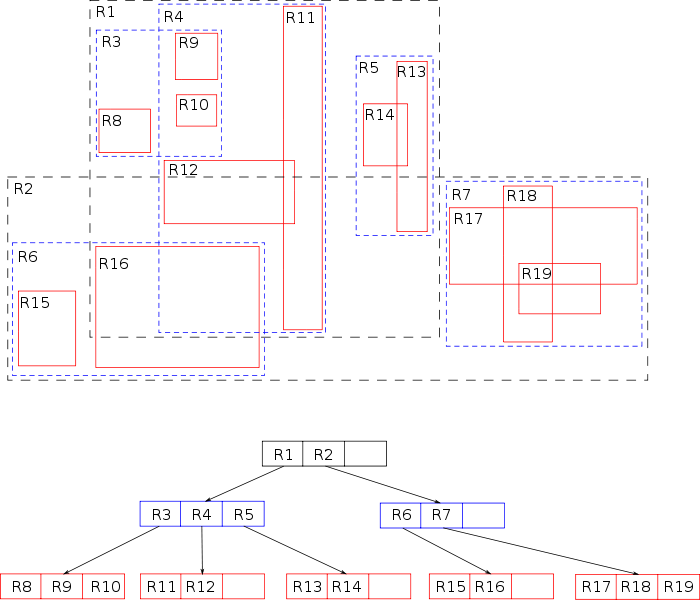
Very shortly said, an R*Tree defines a
tree-like structure based on rectangles (the
R. in R*Tree stands exactly for
Rectangle).
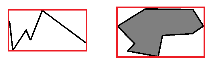
Every arbitrary Geometry can be represented as a
rectangle, irrelevantly of its actual shape: we can simply use the
MBR. (
Minimum Bounding Rectangle) corresponding to such Geometry.
May well be the term
BBOX. (
Bounding Box) is more familiar to you: both terms are exact synonyms.
It's now quite intuitive understanding how the R*Tree does actually works:
- Spatial query defines an arbitrary search frame (this too being a rectangle)
- the R*Tree is quickly scanned identifying any overlapping index rectangle
- and finally any individual Geometry falling withing the search frame will be identified.>
Think of the well known
needle in the haystack problem: using an R*Tree is an excellent solution allowing to find the
needle in a very short time, even when the
haystack actually is an impressively huge one.
Common misconceptions and misunderstandings
“
I have a table storing several zillion points disseminated all around the world:
drawing a map was really painful and required a very long time.
Then I found somewhere some useful hint, so I've created a Spatial Index on this table.
And now my maps are drawn very quickly, as a general case.
Anyway I'm strongly puzzled, because drawing a worldwide map still takes a very long time.
Why the Spatial Index doesn't work on worldwide map ?”
The answer is elementary simple: the Spatial Index can speed up processing only when a small selected portion of the dataset has to be retrieved.
But when the whole (or a very large part of) dataset has to be retrieved, obviously the Spatial Index cannot give any speed benefit.
To be pedantic, under such conditions using the Spatial Index introduces further
slowness, because inquiring the R*Tree imposes a strong overhead.
Conclusion: the Spatial Index isn't a
magic wand. The Spatial Index basically is like a filter.
- when the selected frame covers a very small region of the whole dataset, using the Spatial Index implies a ludicrous gain.
- when the selected region covers a wide region, using the Spatial Index implies a moderate gain.
- but when the selected region covers the whole dataset (or nearly covers the whole dataset), using the Spatial Index implies a further cost.
SQLite's R*Tree implementation details
SQLite supports a first class R*Tree: anyway, some implementation details surely may seem strongly
exotic for users accustomed to other different Spatial DBMS (such as PostGIS and so on).
Any R*Tree on SQLite actually requires
four strictly correlated tables:
- rtreebasename_node stores (binary format) the R*Tree elementary nodes.
- rtreebasename_parent stores relations connecting parent and child nodes.
-
rtreebasename_rowid stores ROWID values connecting an R*Tree node and a corresponding row into the indexed table.
- none of these three tables is intended to be directly accessed: they are reserved for internal management.
-
rtreebasename actually is a Virtual Table, and exposes the R*Tree for any external access.
- important notice: never attempt to directly bungle or botch any R*Tree related table;
quite surely such attempt will simply irreversibly corrupt the R*Tree. You are warned.
SELECT
*
FROM rtreebasename;
| pkuid |
miny |
maxx |
miny |
maxy |
| 1022 |
313361.000000 |
331410.531250 |
4987924.000000 |
5003326.000000 |
| 1175 |
319169.218750 |
336074.093750 |
4983982.000000 |
4998057.500000 |
| 1232 |
329932.468750 |
337638.812500 |
4989399.000000 |
4997615.500000 |
| ... |
... |
... |
... |
... |
Any R*Tree table looks like this one:
- The pkid. column contains ROWID. values.
- minx., maxx., miny. and maxy. defines MBR. extreme points.
The R*Tree internal logic is
magically implemented by the Virtual Table.
SpatiaLite's support for R*Tree
Any SpatiaLite Spatial Index fully relies on a corresponding SQLite R*Tree.
Anyway SpatiaLite smoothly integrates the R*Tree, so to make table handling absolutely painless:
- each time you perform an INSERT., UPDATE. or DELETE. affecting the main table, then SpatiaLite automatically take care to correctly reflect any change into the corresponding R*Tree.
- some triggers will grant such synchronization.
- so, once you've defined a Spatial Index, you can completely forget it.
Any SpatiaLite's Spatial Index always adopts the following naming convention:
- assuming a table named communities. containing the geometry. column.
- the corresponding Spatial Index will be named idx_communities_geometry.
- and idx.communities.pkid. will relationally reference communities.ROWID..
Anyway using the Spatial Index so to speed up Spatial queries execution is a little bit more difficult than in other Spatial DBMS, because there is no tight integration between the
main table and the corresponding R*Tree: in the SQLite's own perspective they simply are two distinct tables.
Accordingly to all this, using a Spatial Index requires performing a
JOIN., and (
may be) defining a
sub-query.
You can find lots of examples about Spatial Index usage on SpatiaLite into the
Haute Cuisine section.
SELECT
CreateSpatialIndex('communities', 'geometry');
-- Add support for SpatialIndex-Queries SELECT
CreateSpatialIndex('populated_places', 'geometry');
This simple declaration is all you are required to specify in order to set a Spatial Index corresponding to some Geometry column. And that's all.
SELECT
DisableSpatialIndex('communities', 'geometry');
And this will remove a Spatial Index:
- please note: this will not DROP. the Spatial Index (you must perform this operation in a separate step).
- anyway related metadata are set so to discard the Spatial Index, and any related TRIGGER. will be immediately removed.
SpatiaLite supports a second alternitive Spatial Index based on MBR-caching.
This one simply is a historical legacy, so using MBR-caching is strongly discouraged.
