SpatiaLite Cookbook Chapter 06: Cooking basics |
Back to the SpatiaLite home page Previous Chapter Chapter 05: Desserts, spirits, tea and coffee Back to the Cookbook home page Next Chapter Chapter 07: Exotic Cooking aspects, which are often forgotten (or avoided)
- List of topics
- An introduction to SpatiaLite
- The OpenGIS geometry model
- Supported spatial data formats
- Coordinate Reference Systems; the EPSG dataset
- Spatial Metadata support
- The VirtualShape module
- The VirtualText module
- Spatial Indexing support
- MBR Caching support
- SpatiaLite conformance and compatibility
- Other topics of interest
|
SpatiaLite is just a small sized SQLite extension. Once you have installed SpatiaLite (a very simple and elementary task), the SQLite DBMS is enable to load, store and manipulate Spatial Data (aka Geographic Data, GIS Data, Cartographic Data, GeoSpatial Data, Geometry Data and alike). SpatiaLite implements spatial extensions following the specification of the Open Geospatial Consortium (OGC), an international consortium of companies, agencies, and universities participating in the development of publicly available conceptual solutions that can be useful with all kinds of applications that manage spatial data. At a very basic level, a DBMS that supports Spatial Data offers an SQL environment that has been extended with a set of geometry types, and thus may be usefully employed i.e. by some GIS application. A geometry-valued SQL column is implemented as a column that has a geometry type. The OGC specification describe a set of SQL geometry types, as well as functions on those types to create and analyze geometry values. The followings are examples of geographic entities with a geometry:
If you are looking for a full fledged Geo-DBMS, capable to support you in every kind of GIS operation, and perhaps for you is paramount to cope with millions and millions of geographic entities, and you are planning to deploy all this in a complex client-server architecture, don't even try to use SpatiaLite + SQLite. Obviously it's not the solution you are looking for; simply it falls too short for your needs. Otherwise, if you are looking for a very basic but full effective desktop Geo-DBMS, with no frills, no undue complexity, and the average volume of your data didn't exceeds a reasonable size, SpatiaLite + SQLite can really be the right solution for your needs. Just to do a very quick comparison with others widely used open source DBMSs supporting Spatial Data:
|
The OpenGIS geometry model in a nutshell
2.1. The geometry class hierarchyThe geometry classes define a hierarchy as follows:
2.2. class GeometryIt is not possible to create objects in non-instantiate-able classes. It is possible to create objects in instantiate-able classes.Geometry is the root class of the hierarchy. It is a non-instantiable class but has a number of properties that are common to all geometry values created from any of the Geometry subclasses. These properties are described in the following list. Particular subclasses have their own specific properties, described later. Geometry PropertiesA geometry value has the following properties:
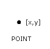
2.3. class PointA Point is a geometry that represents a single location in coordinate space.Point Properties
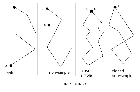
2.4. class CurveA Curve is a one-dimensional geometry, usually represented by a sequence of points. Particular subclasses of Curve define the type of interpolation between points. Curve is a non-instantiable class.Curve Properties
2.5. class LineStringA LineString is a Curve with linear interpolation between points.LineString Properties
2.6. class SurfaceA Surface is a two-dimensional geometry. It is a non-instantiable class. Its only instantiable subclass is Polygon.Surface Properties
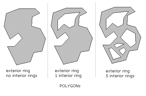
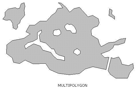
2.7. class PolygonA Polygon is a planar Surface representing a multisided geometry. It is defined by a single exterior boundary and zero or more interior boundaries, where each interior boundary defines a hole in the Polygon.Polygon AssertionsThe boundary of a Polygon consists of a set of LinearRing objects (that is, LineString objects that are both simple and closed) that make up its exterior and interior boundaries.
2.8. class GeometryCollectionA GeometryCollection is a geometry that is a collection of one or more geometries of any class. All the elements in a GeometryCollection must be in the same Spatial Reference System (that is, in the same coordinate system). There are no other constraints on the elements of a GeometryCollection, although the subclasses of GeometryCollection described in the following sections may restrict membership. Restrictions may be based on:
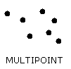
2.9. class MultiPointA MultiPoint is a geometry collection composed of Point elements. The points are not connected or ordered in any way.MultiPoint Properties
2.10. class MultiCurveA MultiCurve is a geometry collection composed of Curve elements. MultiCurve is a non-instantiable class.MultiCurve Properties
2.11. class MultiLineStringA MultiLineString is a MultiCurve geometry collection composed of LineString elements.2.12. class MultiSurfaceA MultiSurface is a geometry collection composed of surface elements. MultiSurface is a non-instantiable class. Its only instantiable subclass is MultiPolygon.MultiSurface Assertions
2.13. class MultiPolygonA MultiPolygon is a MultiSurface object composed of Polygon elements.MultiPolygon Assertions
MultiPolygon Properties
|
Supported spatial data formats
This section describes the standard spatial data formats that are used to represent geometry objects in queries. They are:
Well-Known Text (WKT) formatThe Well-Known Text (WKT) representation of Geometry is designed to exchange geometry data in ASCII form.Examples of WKT representations of geometry objects:
Well-Known Binary (WKB) formatThe Well-Known Binary (WKB) representation for geometric values is defined by the OpenGIS specification. It is also defined in the ISO SQL/MM Part 3: Spatial standard. WKB is used to exchange geometry data as binary streams represented by BLOB values containing geometric WKB information.WKB uses one-byte unsigned integers, four-byte unsigned integers, and eight-byte double-precision numbers (IEEE 754 format). A byte is eight bits. For example, a WKB value that corresponds to POINT(1 1) consists of this sequence of 21 bytes (each represented here by two hex digits): 0101000000000000000000F03F000000000000F03F The sequence may be broken down into these components:
0102000000000000000000F03F000000000000F03F00000000000000400000000000000040 The sequence may be broken down into these components:
010200000001000000000000000000F03F000000000000F03F0100000000000000000000400000000000000040 The sequence may be broken down into these components:
Internal BLOB format
|
|
Each coordinate value, in order to be fully qualified, needs to be explicitly assigned to some SRID, or Spatial Reference Identifier. This value identifies the geometry's associated Spatial Reference System that describes the coordinate space in which the geometry object is defined. As a general rule, different geometries can interoperate in a meaningful way only if their coordinates are expressed in the same Coordinate Reference System. To avoid any confusion, and to grant effective interoperability, SRID values cannot be assigned randomly, but have to adhere to some standard specification as defined by an international authority. The EPSG [European Petroleum Survey Group] is the most authoritative on this field, actually maintaining and distributing a large dataset describing quite any worldwide known Coordinate Reference System. Not only; the EPSG dataset includes Coordinate Transformation geodetic parameters, thus allowing to transform coordinates from some CSR to any other. The followings are examples from the EPSG dataset: You don't have to worry too much about geodetic parameters and their meaning; you simply have to know that the PROJ library can use them the right way in order to transform coordinates between different CSRs. |
|
Basically, a GEOMETRY simply is a glorified kind of BLOB value, implementing an internal structure such as the one we've just seen in the previous chapter. Following such a simplistic approach you can perform some useful tasks. But for sure, this one cannot be the right way to implement a fairly designed and completely reliable Spatial DBMS [i.e. one that is well checked, consistent and properly constrained]. Let we briefly see some horror cases, to better understand which one are the main issues we have to avoid:
And this one is exactly the specific purpose of Spatial Metadata. When you add a GEOMETRY column to some table, you don't simply define it in the most generic way, but you have to specify a GEOMETRY type and a SRID as well. This infos will then be permanently added to Spatial Metadata, and any required constraint will be then enforced each time you'll try to INSERT or UPDATE a row on related table. As defined by OpenGIS specifications, Spatial Metadata are actually implemented as two distinct tables:
And this one is an example from the geometry_columns table:
In the SpatiaLite's own implementation, you are never required to be directly concerned about Spatial Metadata handling. Any related task is automatically performed in a completely transparent way; anything silently happens behind the scenes. The main steps to follow in order to activate all this, are as follows:
|
|
The SQLite DBMS implements a very interesting feature; you can develop some specialized driver in order to access any generic [and possibly exotic] data source, and then those external data will appear to the SQL engine exactly as they where SQLite's native ones. This means you can apply any SQL operation on them, if appropriate / possible and if the driver offers an adequate support. Such mechanism is referred in SQLite's documentation as the VIRTUAL TABLE support; this name is very appropriate, because it allows to access data physically stored anywhere as they where virtually stored in a standard SQLite's table. In a more general way, a VIRTUAL TABLE can hide anything you can think about; it simply represents some software extension module exposing an appropriate interface to the SQLite's database engine, thus allowing standard SQL processing. The VirtualShape module is a VIRTUAL TABLE driver specifically designed to allow direct read only access to shapefiles. The shapefile format is defined by ESRI; you can find a copy of the complete specification at http://www.esri.com/library/whitepapers/pdfs/shapefile.pdf. If you are interested about this argument, you can usefuly read this article: http://en.wikipedia.org/wiki/Shapefile. The ESRI shapefile format is quite obsolescent nowadays, but is still very widely used in GIS, mainly because it is simple, is universal and is supported by any existing GIS software. So it really can be considered as the de facto standard data exchange format for GIS data. VirtualShape is designed to interact very strictly with SpatiaLite, in order to support a complete direct access to shapefiles via standard SQL, for both attributes and geometries. SpatiaLite tools support anyway importing GIS data from shapefiles into spatial tables; but the option to support standard SQL queries directly on external shapefiles, with no need at all to import them in some SQLite table, makes VirtualShape a very valuable module.
|
|
The VirtualText module is another VIRTUAL TABLE driver supporting direct read only access to CSV and TXT-tab files. Formats based on delimited text are widespread; usually you can export quite any kind of tabular data using the CSV or TXT-tab formats. Any mainstream spreadsheet [such as MS Excel or Open Office Calc] supports import / export to and from delimited text. So, adding to SpatiaLite the ability to process on-the-fly this kind of text based formats as they where native SQL data can really be a very useful feature.
Importing a CSV/TXT file seldom can be done automatically
|
|
The SQLite DBMS (as many other DBMS) implements Indices as a mean to quickly retrieve selected data. Imagine a table containing million and million rows, such as the national telephone directory; retrieving the people's name owning some specific telephone number may be a slow operation, if you perform a so called full table scan; i.e. if the DBMS engine has to read and evaluate every row in order to filter the requested one. Implementing an Index on the telephone number column allows for very fast querying; now the DBMS engine can simply read the Index, and immediately will find the required row. There is no need at all to perform the lengthy full table scan process. Please note: if your table contains a limited number of rows (let say 5,000 or 20,000) implementing an Index hasn't any practical effect. SQLite can perform a full table scan in a very short time anyway. But if your table contains an huge number of rows (let say more than 100,000), then implementing an Index can have a dramatic effect on query's execution time. As biggest is the number of rows, as more evident becomes the benefit to implement an Index. The same identical problem arises for Spatial data [i.e. Geometry] as well; but unhappily an ordinary Index cannot be used against a Geometry-type column. This is because ordinary Indices represents an implementation of a so called BTree (i.e. Binary Tree); binary trees can usefully be applied on numbers and / or strings, but not at all on geometries. For geometries we need a completely different kind of Index, i.e. the so called RTree (Rectangle Tree). SQLite's release v.3.6.0 [and the following ones] support a stable and effective implementation for RTRee:
SQLite's RTrees can seem a little bit exotic, but after all they perform very well. From the SpatiaLite perspective, supporting Spatial Indexing via SQLite's RTrees concretely means that:
|
BEWARE:The MbrCache module has deprecated, and is only preserved for continued support of legacy apps.This text will remain available to preserve a full historical record.
All new applications should, instead, use the more recent R*Tree Spatial Index.
The Spatial Index is a complete and more efficient replacement and should now always be used.
Back to the SpatiaLite home page Previous Chapter Chapter 05: Desserts, spirits, tea and coffee Back to the Cookbook home page Next Chapter Chapter 07: Exotic Cooking aspects, which are often forgotten (or avoided)