Back to RasterLite2 doc index
Draping Geometries over DEM/DTM raster grids
or:
How to transform 2D Geometries into 3D ones
A quick introduction
|
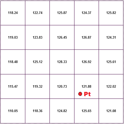
Extrapolating an elevation value (aka Z-coordinate) is straightforward simple in the case of POINT Geometries. We simply have to precisely identify which specific cell of the raster grid is overlapped by the Point. The Z-coord to be set into the Point is the Elevation value assigned to this cell. So, in the example shown by the side figure, Z=121.88 will be set for Point Pt. |
|
|
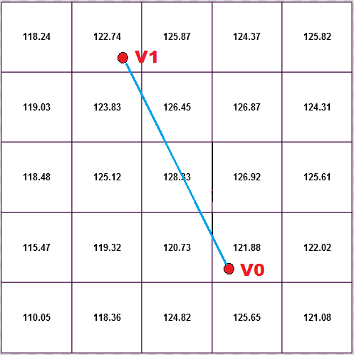
Unhappily things become a little bit more difficult in the case of LINESTRING or POLYGON Geometries. In both this cases we can still continue to adopt the same approach adopted for POINT; we are just required to iteratively loop on each Vertex. But this way, as exemplified by the side figure, we'll get a straight segment connecting V1 to V2 that crosses many cells in the raster grid. If we'll simply ignore at all such cells we'll risk to introduce some kind of information suppression. This can easily cause an unwanted degradation in the accuracy of the interpolated Z-coords, and this surely isn't a good thing. |
|
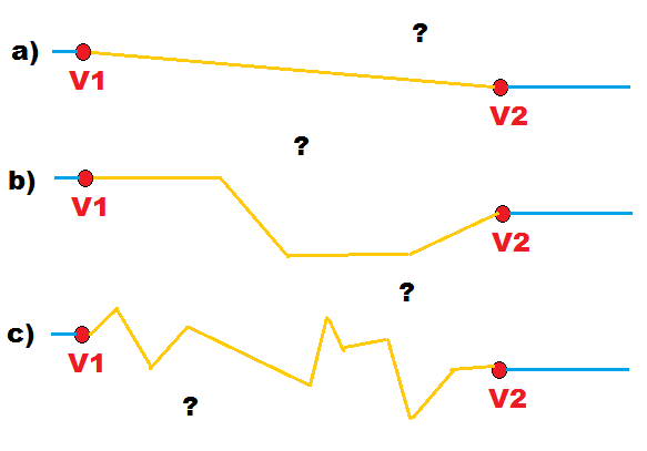
Just to understand better the problem:
|
|
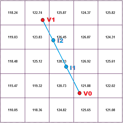
The solution is rather simple:
Warning
|
|
A first practical example
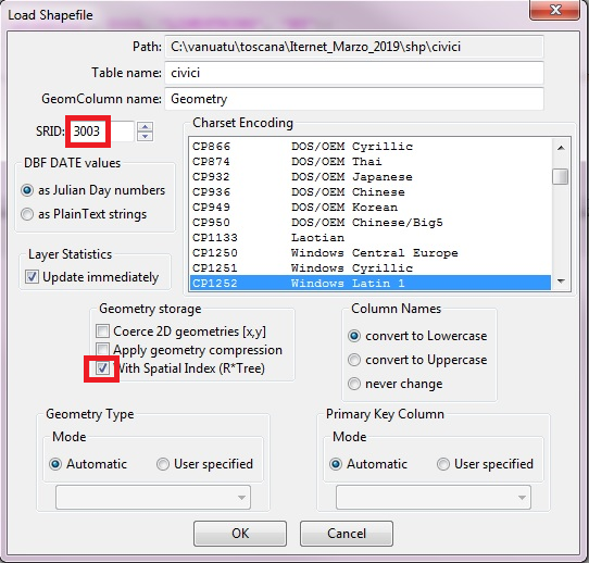
In this first example we'll use the following datasets:- civici.shp: this is a first Shapefile containing more than 1.5 millions of Points (Tuscany House Numbers).
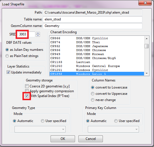
- elem_strad.shp: this is another Shapefile containing more than 400.000 Linestrings (Tuscany Roads).
- dtmoro.asc: an ASCII grid containing a DTM (Digital Terrain Model) covering all Tuscany with a cell resolution of 10m x 10m.
Hint: you'll find both civici.shp and elem_strad.shp within the package named Grafo Stradale (Road Network).
dtmoro.asc is contained within the package named Morfologia / DTM 10x10 Orografico (Morphology / 10x10 Orographic DTM).
step #1: creating and populating the work database
step #1.aFirst of all we'll create and populate the civici Table by importing the corresponding Shapefile (House Numbers).Be sure to set SRID=3003 and to check the option With SpatialIndex (R*Tree). As shown by the side figure we'll use the appropriate GUI wizard for doing this task, but if you wish you could eventually adopt a pure SQL approach by executing the following statement:
SELECT ImportSHP( 'C:\vanuatu\toscana\Iternet_Marzo_2019\shp\civici' ,
       'civici' , 'CP1252' , 3003 , 'Geometry' , 'PK_UID' , 'POINT' , 0 , 0 , 1 , 1 , 'LOWERCASE' );
|
|
step #1.bThen we'll create and populate the elem_civ Table by importing the corresponding Shapefile (Road Network).Be sure to set SRID=3003 and to check the option With SpatialIndex (R*Tree). As shown by the side figure we'll use the appropriate GUI wizard for doing this task, but if you wish you could eventually adopt a pure SQL approach by executing the following statement:
SELECT ImportSHP( 'C:\vanuatu\toscana\Iternet_Marzo_2019\shp\elem_strad' ,
       'elem_strad' , 'CP1252' , 3003 , 'Geometry' , 'PK_UID' , 'LINESTRING' , 0 , 0 , 1 , 1 , 'LOWERCASE' );
|
|
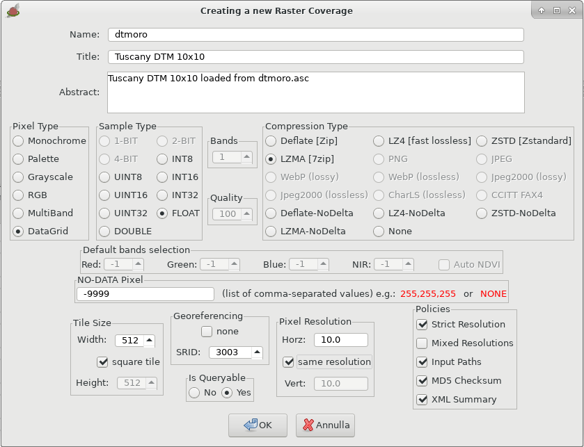
step #1.cNow we'll create an empty Raster Coverage named dtmoro.As shown by the side figure we'll use the appropriate GUI wizard for doing this task, but if you wish you could eventually adopt a pure SQL approach by executing the following statement:
SELECT RL2_CreateRasterCoverage ( 'dtmoro' , 'FLOAT' , 'DATAGRID' , 1 , 'LZMA' , 100 , 512 , 512 , 3003 , 10.0 , 10.0 ,
       RL2_SetPixelValue ( RL2_CreatePixel ( 'FLOAT' , 'DATAGRID' , 1 ) , 0, -9999 ) , 1 , 0 , 1 , 1 , 1 , 1 );
|
|
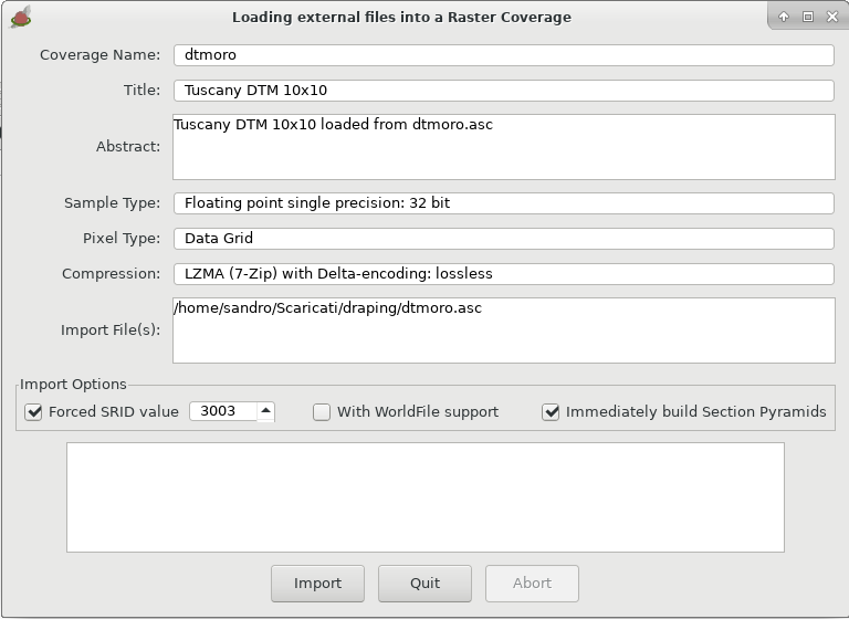
step #1.dAnd finally we'll load the DTM dtmoro.asc into the Raster Coverage created in the previous step.As shown by the side figure we'll use the appropriate GUI wizard for doing this task, but if you wish you could eventually adopt a pure SQL approach by executing the following statement: SELECT RL2_LoadRaster ( 'dtmoro' , '/home/sandro/Scaricati/draping/dtmoro.asc' , 0 , 3003 , 1 , 1 ); |
|
Important notice for Windows usersImporting an ASCII Grid necessarily requires opening a supporting temporary file.Unhappily all recent versions of Windows think that temporary files are dangerous and critical objects raising a serious security alert causing an irreversible error condition. There is only one way allowing to effectively load an ASCII Grid on Windows; the application must necessarily be executed with Administrator privileges. 
|
step #2: transforming a 2D dataset into a 3D one.
All right, now we are finally ready for transforming both civici and elem_strad datasets from 2D into 3D. This task just require executing a single SQL statement:SELECT RL2_DrapeGeometries( NULL , 'dtmoro' , NULL , 'civici' , 'geometry' , 'geom3d' , -9999 , 5.0 , 5.0 , 0 ); --------------------------------------- 1A quick explanation:
- the first argument is the DB-prefix of the attached database containing the DEM/DTM Raster Coverage.
When it's null (as in this case), the MAIN database is always assumed. - the second argument is the Raster Coverage name.
Note that only Raster Coverages of the DATAGRID type can be accepted. - the third argument ... we'll ignore it for now; it will be explained in the second advanced example.
- the fourth argument is the name of the Spatial Table containing the Geometries to be draped, that is always assumed to be in the MAIN database.
Note: both the DTM/DEM Raster Coverage and the Spatial Table must share the same SRID value. - the fifth argument is the name of the 2D Geometry column to be draped.
- the sixth argument is the name of the 3D Geometry column where the result of draping will be stored.
Note: this column must not exist, and will be automatically created by ST_DrapeGeometries() itself. - the seventh argument is the NO-DATA value to assigned as the Z coordinate value to all Points/Vertices of unknown elevation.
Note: in this case we've used -9999, that is the same NoData value we used when creating the Raster Coverage, but you are free to choose any other different value.
There is no relation between the NoData value of the DataGrid and the NoData value of Z-coords. - the eighth argument is the densification distance.
- the ninth argument is the simplification distance.
We have already discussed the scope of both distances in the Introduction; in this case we'll set them accordingly to the Shannon rule (half of the cell resolution).
The DTM has a cell resolution of 10.0 m and consequently setting densification and simplification distances to 5.0 m is surely appropriate. - we'll ignore for now the tenth argument; it will be examined in the Tech Note at the bottom of this Wiki page.
| Table Civici | ||
|---|---|---|
| FID | Geometry (2D XY) | Geom3d (3D XYZ) |
| 1 | POINT(1653899.985931 4755950.991447) | POINT Z(1653899.985931 4755950.991447 39.160851) |
| 139934 | POINT(1733162.94 4816036.29) | POINT Z(1733162.94 4816036.29 257.153503) |
| 1101734 | POINT(1710081.18 4746933.385) | POINT Z(1710081.18 4746933.385 773.801025) |
| Table Elem_Strad | ||
| FID | Geometry (2D XY) | Geom3d (3D XYZ) |
| 7 | LINESTRING(1660575.144841 4862643.223261, 1660539.689436 4862662.612925, 1660498.244354 4862682.023911) |
LINESTRING Z(1660575.144841 4862643.223261 41.513931, 1660539.689436 4862662.612925 41.882999, 1660498.244354 4862682.023911 42.213669) |
| 45155 | LINESTRING(1726222.056843 4821467.815741, 1726222.056843 4821472.627217, 1726221.753693 4821489.603671) |
LINESTRING Z(1726222.056843 4821467.815741 241.396606, 1726222.056843 4821472.627217 241.599594, 1726221.753693 4821489.603671 242.310699) |
| 290805 | LINESTRING(1714208.7 4747016.34, 1714214.75 4747005.98, 1714221.72 4746991.88, 1714225.9 4746983.42, 1714228.21 4746979, 1714231.02 4746973.7, 1714234.47 4746968.2, 1714236.98 4746965.77, 1714241.38 4746961.81, 1714255.92 4746949.84, 1714289.39 4746923.98, 1714301.97 4746914.8, 1714309.22 4746909.2, 1714325.83 4746897.3, 1714355.64 4746875.98) |
LINESTRING Z(1714208.7 4747016.34 968.079285, 1714214.75 4747005.98 966.055481, 1714221.72 4746991.88 962.389526, 1714225.9 4746983.42 959.525391, 1714228.21 4746979 958.444885, 1714231.02 4746973.7 958.444885, 1714234.47 4746968.2 957.226624, 1714236.98 4746965.77 957.226624, 1714241.38 4746961.81 957.226624, 1714255.92 4746949.84 954.927124, 1714289.39 4746923.98 952.606812, 1714301.97 4746914.8 951.481201, 1714309.22 4746909.2 950.266785, 1714325.83 4746897.3 948.182983, 1714355.64 4746875.98 943.776672) |
A second more advanced example
In the first example we've seen that Tuscany has a medium-resolution (10m x 10m cells) DTM.covering the whole surface of the Region.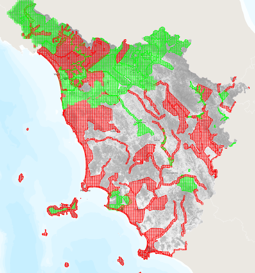
But on many specific areas (shown on the above figure by red and green grids) Tuscany has a second kind of DTM/DSM based on hi-resolution (1m x 1m) Lidar surveys
Such Lidar DTM/DSM don't cover the whole Region, but where they are available they certainly are a source a very valuable elevation data.
Just to add more complications, the Lidar DTM/DSM belongs to two different series (green and red), and are of different ages and accuracy.
The best possible approach for draping Geometries will obviously be the one ensuring that in any case the most recent and accurate elevation data will be used, so to achieve optimal results.
RL2_DrapeGeometries() has the capability to support such a complex scenario, let's see how this is possible.
| How to use multiple Raster Coverages for Draping Geometries | |
|---|---|
| 1 |
In this second example we'll use once again the same civici and elem_strad 2D datasets we've already used in the previous example. And we'll continue to use as before the 10x10 dtmoro so to have an homogeneous DTM covering the whole Region without any gap. |
| 2 | But this time we'll create more Raster Coverages containing all the 1x1 Lidar DTM/DSM that are available. There are many possible ways for doing this, but a good approach would be the one to create a different Raster Coverage for each series and year. e.g. lidar_red_2008, lidar_red_2009, lidar_green_2010, lidar_green_2011 and so on. |
| 3 | Now we have to define an appropriate priority order so to be sure that Draping will then process all Raster Coverages in the required sequence.
|
| 4 | Defining the priority order is rather trivial. You just have to create an helper table like this:
CREATE TEMPORARY TABLE draping_aux (
    progr INTEGER NOT NULL,
    db_prefix TEXT,
    coverage_name TEXT NOT NULL);
--
-- inserting all Lidar Raster Coverages in decreasing priority order
--
...
INSERT INTO draping_aux ( coverage_name , progr ) VALUES ( 'lidar_green_2011' , 10 );
INSERT INTO draping_aux ( coverage_name , progr ) VALUES ( 'lidar_green_2010' , 11 );
INSERT INTO draping_aux ( coverage_name , progr ) VALUES ( 'lidar_red_2009' , 12 );
INSERT INTO draping_aux ( coverage_name , progr ) VALUES ( 'lidar_red_2008' , 13 );
...

--
-- inserting the 10x10 dtmoro Raster Coverage with lowest priority
--
INSERT INTO draping_aux ( coverage_name , progr ) VALUES ( 'dtmoro' , 99 );
Now we are ready for populating the helper table by inserting any required Raster Coverage specifying its relative priority. |
| 5 |
We are finally ready for draping out geometries over multiple Raster Coverages:
SELECT RL2_DrapeGeometries( NULL , NULL , 'draping_aux' , 'civici' , 'geometry' , 'geom3d' , -9999 , 5.0 , 5.0 , 0 );
---------------------------------------
1


SELECT RL2_DrapeGeometries( NULL , NULL , 'draping_aux' , 'elem_strad' , 'geometry' , 'geom3d' , -9999 , 5.0 , 5.0 , 0 );
---------------------------------------
1
These are almost the same calls to RL2_DrapeGeometries() we did in the first example, except for two details:
Useful hintIn order to check the priority order in which the Raster Coverages will be processed by RL2_DrapeGeometries you just have to execute the following SQL query:SELECT db_prefix, coverage_name FROM draping_aux ORDER BY progr; |
| Tech Note: how RL2_DrapeGeometries() internally works |
|---|
|
| Tech Note: draping M-values |
|---|
|
Note: you can eventually use RL2_DrapeGeometries() so to set M-values instead of Z-values. Quick recall: by definition M-values are intended to support any possible kind of generic measures.This exactly is the same definition adopted by generic DataGrids. So RL2_DrapeGeometries() can be legitimately called for interpolating M-values instead of Z-values whenever you'll think it could be useful. Just few practical examples: think of some DataGrid containing temperature or rain intensity or wind speed or noise intensity or population density measures. In all these cases you could probably find useful interpolating such measures as M-values directly stored in your Geometries. SELECT RL2_DrapeGeometries( NULL , 'dtmoro' , NULL , 'civici' , 'geometry' , 'geom3d' , -9999 , 5.0 , 5.0 , 1 ); --------------------------------------- 1
|
Back to RasterLite2 doc index