Tessellation-related SQL functions supported in version 4.0.0
backGeneralities about tessellations
Tessellation is the process of creating a two-dimensional plane using the repetition of a geometric shape with no overlaps and no gaps. read moreA tessellation could be eventually based on identical cells, all of exactly the same shape and size. In this case we'll have a regular tessellation.
Just a quick recall of elementary geometry; there are simply 3 regular polygonal shapes we can use in order to get a regular tessellation: the equilateral triangle, the square and the regular hexagon.
On the other way many tessellations aren't regular at all, because each single cell has an individual size and shape of its own.
It's really interesting to note that many natural shapes closely resemble a tessellation: going from biology to crystallography since geology and landscapes it's not at all difficult to identify many natural tessellation examples on the wild. So it's not at all surprising to discover that tessellations are often useful in geography as well.
Setting up a testbed DB
In this short tutorial we'll use a very simple SpatiaLite DB, just containing the following Geometry tables:- Administrative boundaries for Italy regions: you can download this dataset from ISTAT (released on CC-BY license terms).
- Main Italian populated places (namely, Local Councils): you can download this dataset from GeoNames (released on CC-BY license terms).
Please note: this one is a worldwide dataset; italian populated places have then been extracted imposing the SQL clause
WHERE county_code = 'IT' AND population > 0
Just to keep any example as simple as possible, both datasets have been referenced into the SRID=23032 - ED50 / UTM zone 32 N
Creating regular tessellations in Spatial SQL
| ||
using Square cells
This SQL query will return a regular grid (square cells) covering Tuscany (cod_reg=9). Each grid's cell will have an edge length of exactly 10 Km |
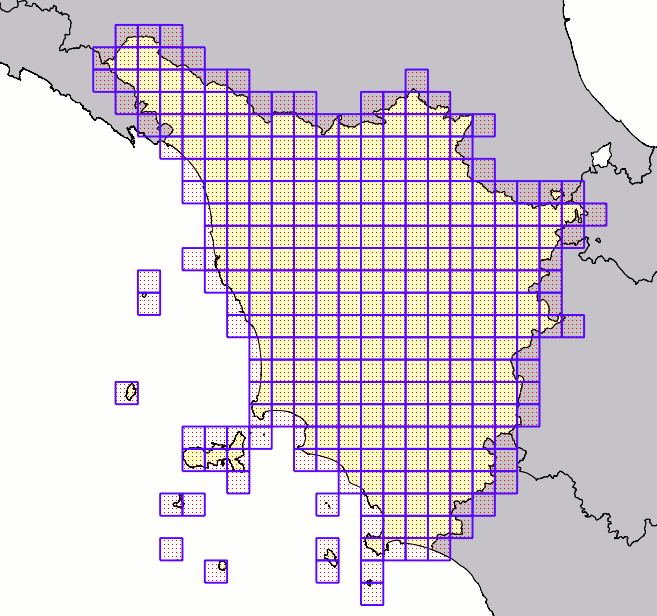 | |
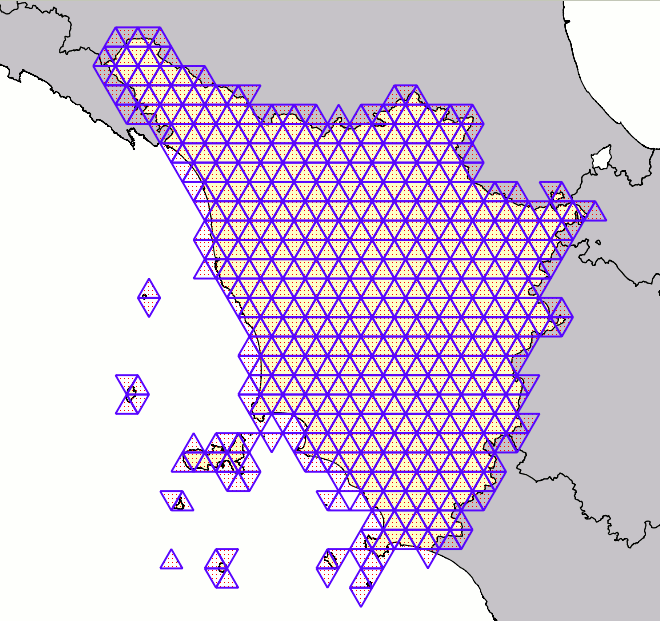
using Triangular cells
|
 | |
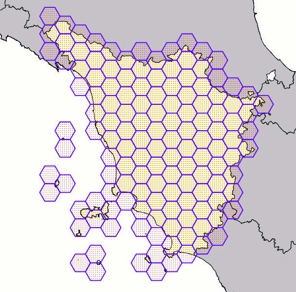
using Hexagonal cells
|
 | |
Delaunay Triangulations
Triangulations simply represent a special case of tessellations: in this case all cells are represented by generic triangles, not necessarily of the equilateral kind.A Delaunay Triangulation is very peculiar because a specific constraint is imposed.
All triangles in a Delaunay triangulation must satisfy the empty circle property: i.e. for each edge we can find a circle containing the edge's endpoints but not containing any other points. read more
Computing a Delaunay Triangulation representing many points is a very complex operation, and one possibly imposing a huge computational load and may be requiring a long time. Happily enough many highly efficient algorithms have been already developed for the Delaunay problem.
The next-to-come GEOS 3.4.0 will support Delaunay Triangulations; this GEOS version is currently still under active development, but the experimental base-code (trunk) seems to be stable enough to be safely tested. SpatiaLite already relies on GEOS for many tasks, so integrating a smooth support for Delaunay Triangulation as well wasn't at all difficult.
|
prototype: ST_DelaunayTriangulation( input Geometry ) : delaunay Geometry ST_DelaunayTriangulation( input Geometry, edges_only boolean ) : delaunay Geometry ST_DelaunayTriangulation( input Geometry, edges_only boolean, tolerance double precision ) : delaunay Geometry |
- the input Geometry can be of absolutely arbitrary type; all Linestrings and / or Polygowns will eventually be dissolved into Points corresponding to vertices.
So after all ST_DelaunayTriangulation() will always process a MultiPoint. - the optional edges_only argument will be interpreted as follows:
- if FALSE (default value) a MultiPolygon will be returned.
- if TRUE a MultiLinestring will be returned (simply representing the triangles edges).
- the optional tolerance argument is intended to normalize the input point-set, suppressing repeated (or too much close) points. By default a 0.0 tolerance will be assumed.
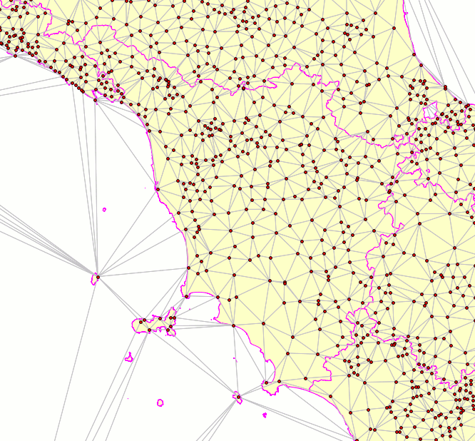
This SQL query will return a Delaunay Triangulation based on Italy's populated places (about 8,000+ Points). The visual example simply covers Tuscany, so the ensure an easy readability. |
 |
Voronoj Diagrams
|
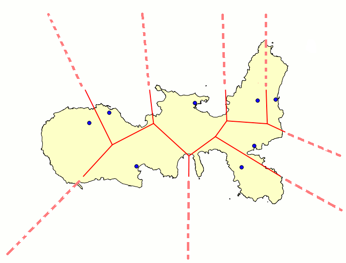
The Voronoj Diagram simply is the dual graph of the Delaunay Triangulation.
A Voronoj Diagram still is a tessellation, and cells in a Voronoj can have any arbitrary polygonal (irregular) shape. This figure clearly shows the relation joining the Delaunay Triangulation and the corresponding Voronoj Diagram. Each single Voronoj's cell is obtained by connecting all the circumcenters of adjacent Delaunay's triangles; consequently each Voronoj cell surely contains one (and only one) Delaunay's node. The cell in the Voronoj Diagram presents an interesting property: all points falling within the same cell are ensured to be nearest to the Delaunay's node placed on the cell itself than to any other Delaunay's node placed in a different cell. So the Voronoj Diagram is a very effective conceptual tool allowing to divide an arbitrary space region into many rationally defined cells, and is thus widely used on many applicative fields based on Computational Geometry. This obviously including Geography itself. read more |
|
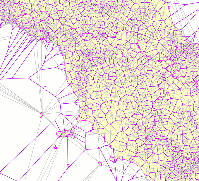
Please note: any Voronoj Diagram will always present an unpleasant complication; when reaching the exterior boundary of the input point-set, there aren't enough points allowing to properly close a cell. And consequently many cells laying near to the exterior boundary actually are open cells, presenting edges going directly to the infinite. The directions of such edges are absolutely well determined; but assigning them a finite length isn't allowed at all. And consequently isn't possible defining a polygon representing these cells. This figure shows a limited Voronoj Diagram always based on the same dataset as above, but this time including only Populated Places laying on the Island of Elba. |
|
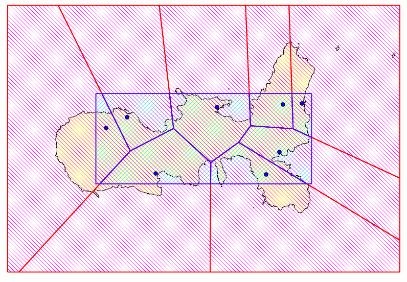
Anyway we can usefully apply a trick effectively allowing to ensure that all cells in a Voronoj will be properly closed. We simply have to constrain the Voronoj Diagram within a rectangular frame of arbitrary size, then computing the intersections between infinite lines and the frame itself. This figure shows the same Voronoj as before, this time opportunely framed; as you can easily notice, now all cells are surely closed and can be safely be represented by a well defined polygon. The size (aka extent) of the frame is absolutely arbitrary, and can be freely set as you wish better accordingly to your specific requirements. Please notice: the blue and the red frame have a strongly different extent, but both them have the same identical overall shape. |
|
prototype: ST_VoronojDiagram( input Geometry ) : voronoj Geometry ST_VoronojDiagram( input Geometry, edges_only boolean ) : voronoj Geometry ST_VoronojDiagram( input Geometry, edges_only boolean, extra_frame_size double precision ) : voronoj Geometry ST_VoronojDiagram( input Geometry, edges_only boolean, extra_frame_size double precision, tolerance double precision ) : voronoj Geometry |
- the input Geometry can be of absolutely arbitrary type; all Linestrings and / or Polygowns will eventually be dissolved into Points corresponding to vertices.
So after all ST_VoronojDiagram() (exactly as ST_DelaunayTriangulation) will always process a MultiPoint. - the optional edges_only argument will be interpreted as follows:
- if FALSE (default value) a MultiPolygon will be returned.
- if TRUE a MultiLinestring will be returned (simply representing the triangles edges).
- the optional extra_frame_size allows to freely set the extent of the frame.
This argument is intended as a percent increase of the natural extent of Voronoj as determined by evaluating all Delaunay's nodes and circumcenters.
By default a 5% extra_frame_size is assumed. - the optional tolerance argument is intended to normalize the input point-set, suppressing repeated points (simply used when internally computing the Delaunay Triangulation). By default a 0.0 tolerance will be assumed.
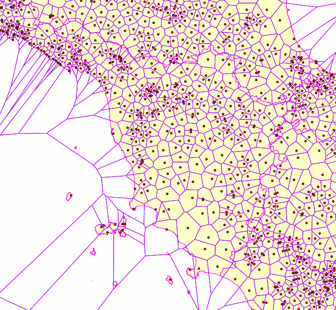
This SQL query will return a Voronoj Diagram based on Italy's populated places (about 8,000+ Points). The visual example simply covers Tuscany, so the ensure an easy readability. All populated places (aka cell seeds) are explicitly represented. |
 |
Delaunay Triangulation, Convex Hull and Concave Hull
|
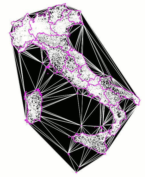
An interesting point absolutely worth to be explicitly noted: the boundary of any Delaunay Triangulation exactly corresponds to the Convex Hull for the same input Geometry.
read more And this in turn opens the way to a further consideration: we could purposely simplify a Delaunay Triangulation so to get a concave hull. You can get more extensive informations about this approach from here Please note well: the convex hull concept corresponds to a robust and formal mathematical definition. On the other side the concave hull is a much more vague and undetermined notion. There is one and only one ConvexHull for a given Geometry; but many ConcaveHulls are possible. Choosing the one or the other is much more a matter of personal taste than a mathematical operation formally defined. Computing a ConcaveHull always is an inherently arbitrary and heuristic process. |
The SpatiaLite's own approach to ConcaveHull
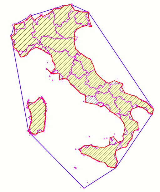
Adopting a very high factor value practically means applying a very bland filtering (very few triangles will be discarded, and you'll consequently get a rather convex shape). On the other side adopting a very low factor values will apply a very strong filtering (many triangles will be now discarded, and you'll get a very concave shape). Useful constants: assuming a perfectly normal distribution of edge lengths (a by far unrealistic assumption for real world datasets), 3σ will imply suppressing about 0.1% triangles (only the few ones presenting abnormally lengthy edges), 2σ corresponds to about 2.1%, and 1σ roughly corresponds to 15.8%. Usually values ranging between 3σ and 2σ are the most appropriate to be used. The figure shows what you can actually get by applying a 3σ filtering to Italian Populated Places; for clarity all Italian Regions are represented in yellow, and the ConvexHull is represented in blue. The ConcaveHull itself is represented in red. |
|
Please note well: PostGIS supports its own implementation of ST_ConcaveHull(), being based on a completely different approach. You can get more details from here
Please, don't be confused: the SpatiaLite and PostGIS implementations are completely unrelated. Anyway, it could be interesting noting that the SpatiaLite's own implementation seems to be much more efficient and fast, and can be realistically applied even to very huge point-sets.
|
prototype: ST_ConcaveHull( input Geometry ) : concave Geometry ST_ConcaveHull( input Geometry, factor double precision ) : concave Geometry ST_ConcaveHull( input Geometry, factor double precision, allow_holes boolean ) : concave Geometry ST_ConcaveHull( input Geometry, factor double precision, allow_holes boolean, tolerance double precision ) : concave Geometry |
- the input Geometry can be of absolutely arbitrary type; all Linestrings and / or Polygowns will eventually be dissolved into Points corresponding to vertices.
So after all ST_ConcaveHull() (exactly as ST_DelaunayTriangulation) will always process a MultiPoint. - the optional factor is intended to be a σ multiplier, thus determining the filtering threshold.
By default a 3σ factor is assumed. - the optional allow_holes argument will be interpreted as follows:
- if FALSE (default value) any eventual interior hole will be suppressed.
- if TRUE any eventual interior holes will be preserved.
- the optional tolerance argument is intended to normalize the input point-set, suppressing repeated points (simply used when internally computing the Delaunay Triangulation). By default a 0.0 tolerance will be assumed.
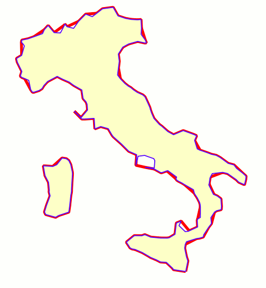
This SQL query will return a ConcaveHull based on Italy's populated places (about 8,000+ Points) by applying a 2.5σ filtering factor. The figure also shows the ConcaveHull returned by the previous example by applying a 3σ factor (red boundary), so to evidentiate the relative differences. |
 |
back