A first, simple and very inefficient, approach
SELECT geonameid, name, country,
    Min(ST_Distance(MakePoint(10, 43), geom, 1)) / 1000.0 AS dist_km
FROM airports;
--------------------------------
6299623	| Marina Di Campo | IT | 33.043320

SELECT geonameid, name, country,
    Min(ST_Distance(MakePoint(10, 43), geom, 1)) / 1000.0 AS dist_km
FROM airports
WHERE geonameid NOT IN (6299623);
---------------------------------
6299392 | Bastia-Poretta | FR | 65.226573

SELECT geonameid, name, country,
    Min(ST_Distance(MakePoint(10, 43), geom, 1)) / 1000.0 AS dist_km
FROM airports
WHERE geonameid NOT IN (6299623, 6299392);
---------------------------------
6299628 | Pisa / S. Giusto | IT	| 82.387014

SELECT geonameid, name, country,
    Min(ST_Distance(MakePoint(10, 43), geom, 1)) / 1000.0 AS dist_km
FROM airports
WHERE geonameid NOT IN (6299623, 6299392, 6299628);
---------------------------------
6299630 | Grosseto Airport | IT | 91.549773

SELECT geonameid, name, country,
    Min(ST_Distance(MakePoint(10, 43), geom, 1)) / 1000.0 AS dist_km
FROM airports
WHERE geonameid NOT IN (6299623, 6299392, 6299628, 6299630);
---------------------------------
6694495 | Corte | FR | 102.819778
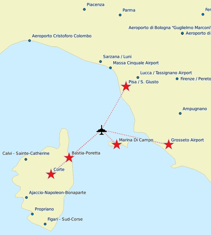
We could effectively execute a first SQL query using the Min() aggregate function in order to identify the closest airport to an arbitrary position (latitude=43.0, longitude=10.0) located in the middle of the Tyrrhenian Sea.Then we could continually repeat the identical query, each time excluding all airports we've already identified in the previous processed steps. The final result will be a full list of the first five airports closest to the reference location ordered by increasing distance.
Such a simple approach is highly impractical, because it strictly requires to hand-write several ad hoc SQL queries one by one. Writing a fully automated SQL script isn't at all a simple task, and some kind of higher level scripting (e.g. Python) would be easily required in any realistic scenario. The automation of all required SQL queries isn't the most critical issue we have to face; the real, critical, bottleneck with this simple approach, is that each of these queries will cause an awful full table scan This will be the cause of an intolerably sluggish performance, and the overall performance will quickly become worse as the dataset progressively increases in size. Conclusion: Some easier and smarter approach is required: possibly one taking full profit from an R*TRee Spatial Index supporting the Geometries to be searched. VirtualKNNStarting with version 4.4.0 SpatiaLite supports a VirtualKNN Virtual Table specifically intended as a complete and highly efficient solution to the KNN problem.CREATE VIRTUAL TABLE knn USING VirtualKNN();Every new db-file being created with 4.4.0 will always automatically define a KNN virtual table. On any earlier version of a SpatiaLite db-file, you can add the KNN support by manually executing the above SQL statement. Note: VirtualKNN necessarily requires 4.4.0 binary support, so any attempt to open a db-file including a VirtualKNN table by using some previous version (<= 4.3.0a) will surely raise an error condition. A first basically simple KNN querySELECT * FROM knn WHERE f_table_name = 'airports' AND ref_geometry = MakePoint(10, 43);
A second sample of a more sophisticated KNN querySELECT a.pos AS rank, b.geonameid, b.name, b.country, a.distance / 1000.0 AS dist_km FROM knn AS a JOIN airports AS b ON (b.geonameid = a.fid) WHERE f_table_name = 'airports' AND ref_geometry = MakePoint(10, 43) AND max_items = 5;
This second KNN query will return the same identical results we already received before by using the simple approach. The striking difference is that this KNN query successfully completes in just a fraction of a second, while executing the first inefficient queries required many seconds (and that with a relatively small dataset). Summary: KNN queries are really efficient and fast, because they directly interact with the lowermost levels of the R*Tree Spatial Index implementation. A third sample of KNN querySELECT a.pos AS rank, b.geonameid, b.name, b.country, a.distance / 1000.0 AS dist_km FROM knn AS a JOIN airports AS b ON (b.geonameid = a.fid) WHERE f_table_name = 'airports' AND ref_geometry = MakePoint(-17.3, -44) AND max_items = 5;
This last KNN query is very similar to the previous one. This time we've placed the origin location somewhere in the blue deep waters of the South Atlantic (more or less midway between Brazil and South Africa) and consequently the nearest airports are not really so near, because they are located many thousands of Kilometers away. As you can easily check by yourself a KNN query will efficiently perform even under such unusual conditions. 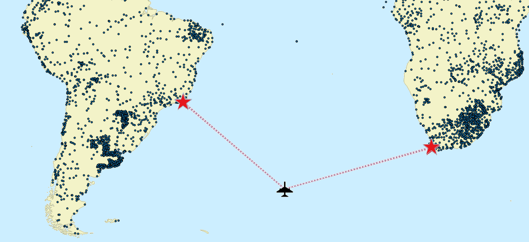 Summary: KNN queries never assume any predefined distribution of the searched items, and will extract the correct results (sorted by distance), despite the very irregular sample distribution. Advanced tutorialYou can download the sample db-file used in the samples of this advanced tutorial.This is a much more demanding dataset with a collection of about 2.4 million house numbers. The original input shapefile was downloaded from Tuscany Region (Grafo Stradale civici.shp) and was subsequently rearranged into a more convenient form. The dataset is released under the CC-BY-SA 4.0 license terms. The used reference system is 3003 Monte Mario / Italy zone 1; this is a planar (projected) reference system measured in meters.
SELECT a.pos AS rank, a.fid AS fid, a.distance AS dist_m, d.prov AS province,
       d.nome AS municipality, c.toponimo AS street_name, b.civico AS house_num,
       b.geom AS geom
FROM knn AS a
JOIN civici AS b ON (b.rowid = a.fid)
JOIN toponimi AS c ON (c.fid = b.id_toponimo)
JOIN comuni AS d ON (d.fid = c.id_comune)
WHERE a.f_table_name = 'civici' AND a.ref_geometry = MakePoint(1733003, 4816332, 3003) AND a.max_items = 10;

SELECT a.pos AS rank, a.fid AS fid, a.distance AS dist_m, b.prov AS province,
       b.comune AS municipality, b.toponimo AS street_name, b.civico AS house_num,
       b.geom AS geom
FROM knn AS a
JOIN vw_civici AS b ON (b.rowid = a.fid)
WHERE a.f_table_name = 'vw_civici' AND a.ref_geometry = MakePoint(1733003, 4816332, 3003) AND a.max_items = 10;
The following map corresponds to the above queries: the origin point is positioned on a road junction in the central area of a densely populated town (Arezzo).Not surprisingly the ten nearest house numbers have been located within a radius of about 10m. 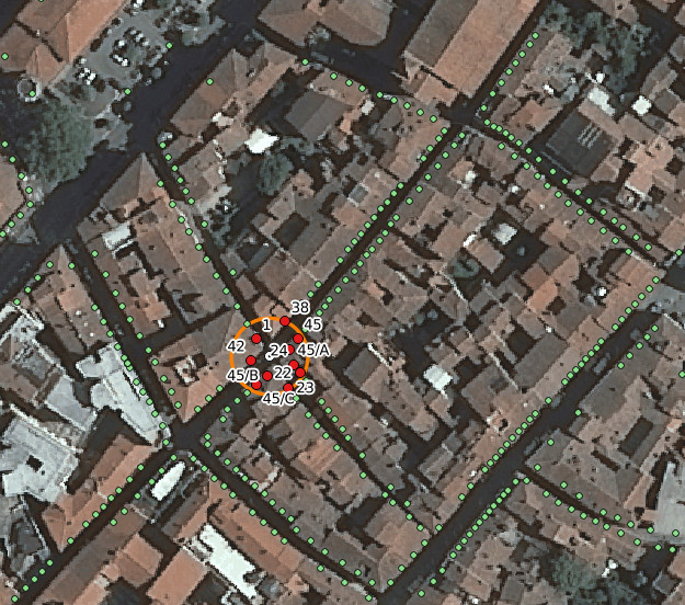
Both queries will return identical results. A closer look will show you that the second query is based on a Spatial View Summary: a VirtualKNN query can indifferently target either a GeoTable or a properly registered Spatial View.
SELECT a.pos AS rank, a.fid AS fid, a.distance AS dist_m, b.prov AS province,
       b.comune AS municipality, b.toponimo AS street_name, b.civico AS house_num,
       b.geom AS geom
FROM knn AS a
JOIN vw_civici AS b ON (b.rowid = a.fid)
WHERE a.f_table_name = 'civici' AND a.ref_geometry = MakePoint(1595625, 4767420, 3003) AND max_items = 20;
The following map corresponds to the above query. Now the origin point is positioned in the Tyrrhenian Sea, about 26 km from the Tuscany mainland and the Islands of Elba and Capraia.Here too VirtualKNN is capable of identifying the nearest house numbers in just a fraction of a second. 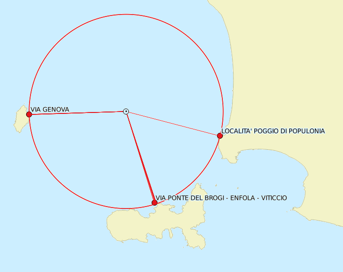 Summary: VirtualKNN is highly efficient and very fast. Even when querying such a huge dataset, while exploring the most contrasting (very high / low density) data distributions .
| ||||||||||||||||||||||||||||||||||||||||||||||||||||||||||||||||||||||||||||||||||||||||||||||||||||||||||||||||||||||||||||||||||||||||
KNN
Not logged in