Importing and exporting geospatial data as CAD drawing files
Starting since version 4.1.0 SpatiaLite supports the capability to read and write external DXF files.Just a very quick introduction: DXF files are commonly used to exchange technical and engineering drawings. It's a very popular and widely adopted format; it's the de-facto data exchange standard format supported by practically all CAD-oriented software applications. Any DXF file simply is a structured text file, so it's not at all platform-specific.
The DXF format was initially invented by Autodesk so to allow an easy and open cross-interoperability between their own AutoCAD and other third-party CAD applications. Many subsequent versions of the DXF format specification appeared during the recent past, but all them share the same basic conceptual layout. As long as Autodesk will continue to freely publish the updated DXF format specifications (as it actually was during the last two decades) we can safely assume that DXF is a reasonably open exchange format.
The DXF format is obviously oriented toward the CAD environment; anyways it's not at all surprising to discover that DXF files are very often used even on GIS/GeoSpatial environments. Both for CAD and GIS the common technological background is represented by vector graphics; so it's not at all surprising to discover that a common overlapping area exist joining both worlds. You can easily discover that in many cases geographic maps are rather indifferently shipped e.g. as ESRI Shapefiles or as Autodesk DXF files.
You should always pay close attention to a really important aspect: CAD and GIS paradigms are substantially different under many ways, so you can never reasonably expect a perfect 1:1 conceptual mapping between both them. Anyway, a limited and constrained cross-operability between CAD and GIS data is allowed, as far as the the main goal is sharing primitive geometries, i.e. points, lines and polygons.
The DXF support implemented in SpatiaLite 4.1.0 doesn't pretend at all to cover any possible CAD-specific facet, this including the fanciest ones.
The intended scope simply is to implement a very basic, unsophisticated and really crude minimal interoperability core: just as strictly indispensable so to allow importing and exporting reasonably structured geographic maps and mainly focusing on basic primitive geometries: no more than this, no less than this.
Useful resources for testing purposes
There are many download sites placed at the four corners of the world offering DXF maps; anyway, the following ones are few URLs you can use for your first tests.http://www.sit.comune.parma.it/ComuneParma/Cartografia%20vettoriale.aspx?idArea=2&idElenco=69 http://urp.comune.bologna.it/PortaleSIT/portalesit.nsf/ViewDocWeb/BF4C7265DF03ACBEC12577A00046C716?OpenDocument http://www.cadforum.cz/catalog_en/?cat=81&page=3 http://gis.sedgwick.gov/dxf/twnshpdxf.asp
Importing DXF maps on spatialite_gui
For this first example we'll use Wichita Township's Parcel Data.
http://gis.sedgwick.gov/dxf/twnshpDXF.asp?08widxfWichita
step#1 - downloading the DXF input filesNow you have to create a new (possibly empty) folder, then saving into it the following DXF files you'll download:http://gis.sedgwick.gov/pub/Aerials/section/wi27s1e/wi01lb.dxf http://gis.sedgwick.gov/pub/Aerials/section/wi27s1e/wi02lb.dxf http://gis.sedgwick.gov/pub/Aerials/section/wi27s1e/wi03lb.dxf http://gis.sedgwick.gov/pub/Aerials/section/wi27s1e/wi04lb.dxf http://gis.sedgwick.gov/pub/Aerials/section/wi27s1e/wi05lb.dxf http://gis.sedgwick.gov/pub/Aerials/section/wi27s1e/wi06lb.dxf http://gis.sedgwick.gov/pub/Aerials/section/wi27s1e/wi07lb.dxf http://gis.sedgwick.gov/pub/Aerials/section/wi27s1e/wi08lb.dxf http://gis.sedgwick.gov/pub/Aerials/section/wi27s1e/wi09lb.dxf http://gis.sedgwick.gov/pub/Aerials/section/wi27s1e/wi10lb.dxf http://gis.sedgwick.gov/pub/Aerials/section/wi27s1e/wi11lb.dxf http://gis.sedgwick.gov/pub/Aerials/section/wi27s1e/wi12lb.dxfIf you wish you could eventually download even more DXF files; anyway the above selection is a good realistic staring point. step#2 - inserting a custom Reference SystemThe Spatial Reference System adopted by these Parcel Data seems to be NAD 1983 StatePlane Kansas South FIPS 1502 Feet; such SRS isn't currently supported between the standard ones, so you are now required to manually insert this custom definition:
INSERT INTO spatial_ref_sys (srid, auth_name, auth_srid, ref_sys_name, proj4text)
VALUES (102678, 'ESRI', 102678, 'NAD 1983 StatePlane Kansas South FIPS 1502 Feet',
    '+proj=lcc +lat_1=37.26666666666667 +lat_2=38.56666666666667 +lat_0=36.66666666666666 ' ||
    '+lon_0=-98.5 +x_0=399999.9999999999 +y_0=399999.9999999999 +ellps=GRS80 ' ||
    '+datum=NAD83 +to_meter=0.3048006096012192 +no_defs');
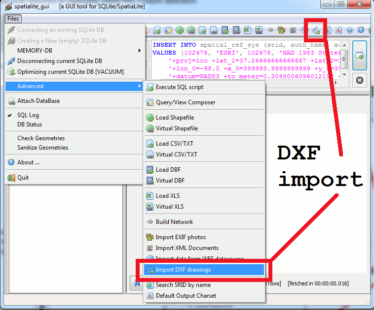
All right: now you are ready to import all DXF maps into a SpatiaLite DB. | |
| You can start a DXF import session indifferently from the main menu or by pressing the corresponding toolbar button. |
|
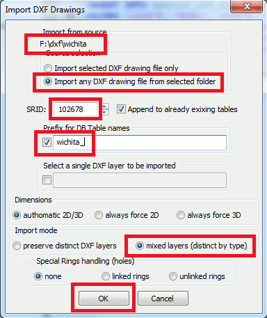
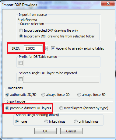
Now you simply have to set few import options as more appropriate:
|
|
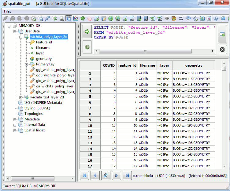
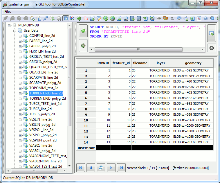
| As you can easily verify, after importing DXFs now two new DB tables have been created. Please note: there are absolutely no lines within Wichita's Parcel Data; this is very uncommon and rather exceptional. A single DB table will now contain any imported geometry of the polygon type. Anyway the DXF import tool has carefully preserved a full track of both the origin file and the corresponding DXF layer. |
|
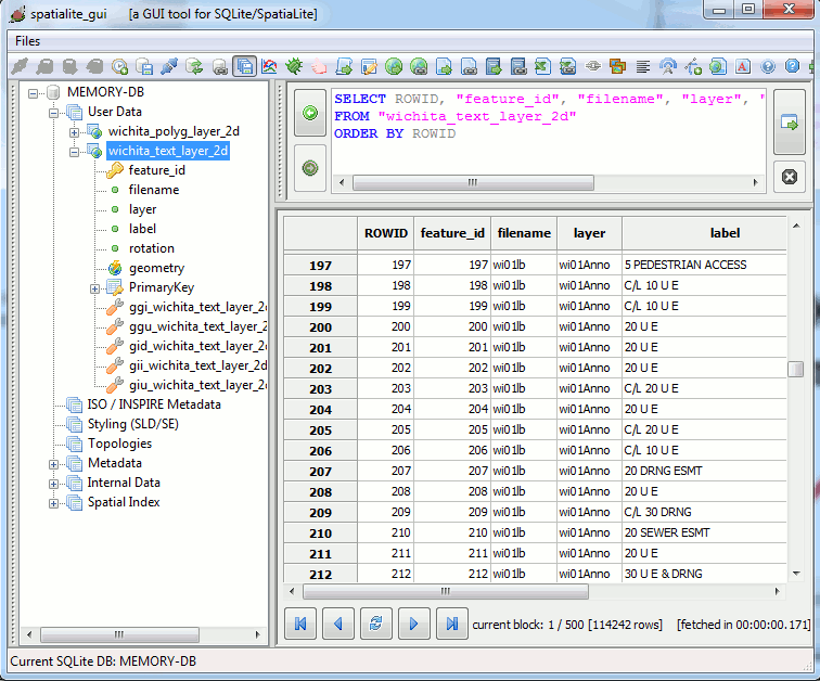
| A second DB table now contains all text labels; this kind of feature has no direct equivalent in GeoSpatial terms. It basically corresponds to a point geometry associated with a text label and a rotation angle. |
|
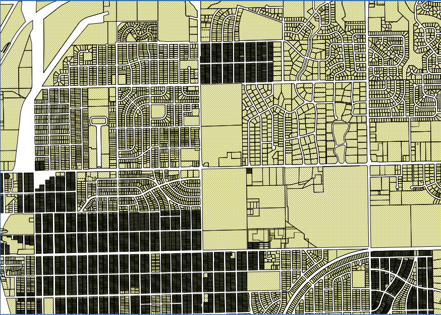
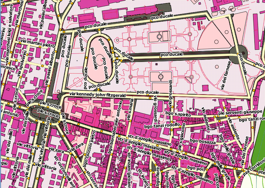
| this is a medium scale screenshot of the imported map as rendered by QGIS |
|
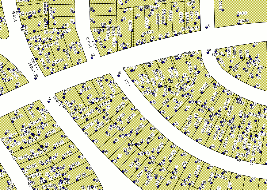
| and here is an enlarged map detail of Wichita's Parcel Data |
|
In this second example we'll use Parma DXF maps.
http://www.sit.comune.parma.it/ComuneParma/Cartografia%20vettoriale.aspx?idArea=2&idElenco=69
Downloading the DXF input filesYet again, you have to create a new (possibly empty) folder, then saving into it the following DXF files you'll download:http://www.sit.comune.parma.it/cgi-bin/files/2012/DXF_Tavole/20.zip http://www.sit.comune.parma.it/cgi-bin/files/2012/DXF_Tavole/21.zip http://www.sit.comune.parma.it/cgi-bin/files/2012/DXF_Tavole/22.zip http://www.sit.comune.parma.it/cgi-bin/files/2012/DXF_Tavole/23.zip http://www.sit.comune.parma.it/cgi-bin/files/2012/DXF_Tavole/26.zip http://www.sit.comune.parma.it/cgi-bin/files/2012/DXF_Tavole/27.zip http://www.sit.comune.parma.it/cgi-bin/files/2012/DXF_Tavole/28.zip http://www.sit.comune.parma.it/cgi-bin/files/2012/DXF_Tavole/29.zipYou could eventually download even more DXF files; and finally you'll be able to start importing all DXF maps into a SpatiaLite DB. | |
Exactly as before, you simply have to set few import options:
|
|
| As you can easily check, this second DXF import has now created an impressive number of new DB tables. Please note: one of most relevant differences between GIS and CAD layers is in that the same CAD layer can easily contain many different kind of Geometries. This is absolutely not allowed under the more strict GIS/GeoSpatial requirements, where each single layer absolutely has to contain Geometries of the same identical type and dimension. So a rather impressive proliferation of many different DB tables is what you can reasonably expect while importing DXF data fully respecting the original layers' layout. |
|
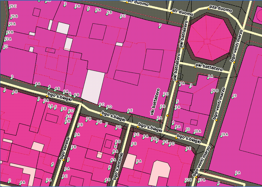
| this is a medium scale screenshot of the imported map as rendered by QGIS |
|
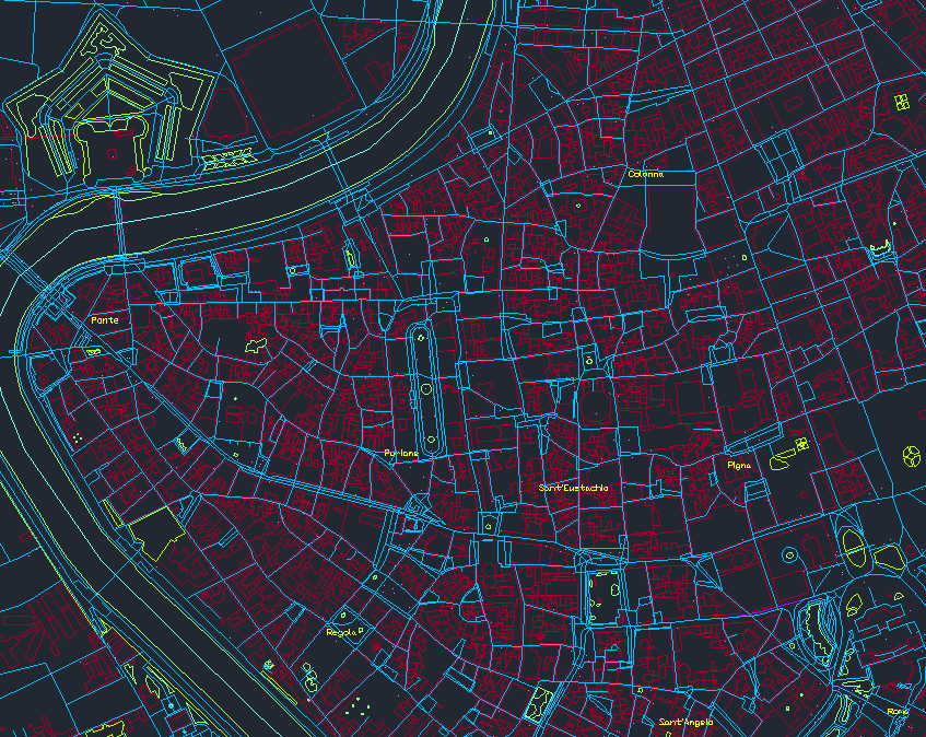
| and here is an enlarged map detail of the Old Town, just near the wonderful Baptistery of Parma. |
|
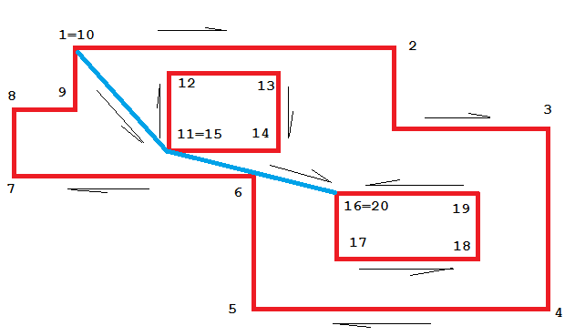
Special Rings Handling (holes)A striking difference between CAD and GIS Geometries is the one related to Polygon's interior rings (aka holes).
Accordingly to all this, many users / organizations have invented during the past years some useful conventional trick allowing to translate GIS Polygons into CAD Polylines (and the opposite) still continuing to fully preserve all holes without any information loss. It looks like the two following criteria are rather popular:
| |
Unlinked Rings
|
|
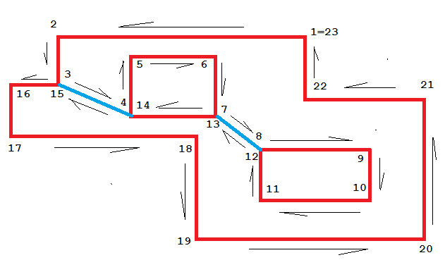
Linked Rings
|
|
Importing DXF maps using the command line tool
More or less the same identical support for DXF import is made available on the Command Line Tool as well.In this case you simply have to invoke the .loaddxf macro dot command by passing the appropriate arguments.
.loaddxf <args>   Loads data from some DXF source into SpatiaLite tables
                  arg_list: DXF_path [srid] [append] [dims] [mode]
                      [rings] [table_prefix] [layer_name]
                  append={Y|N} dims={AUTO|2D|3D} mode={DISTINCT|MIXED}
                  rings={NONE|LINKED|UNLINKED}
Please note: .loaddxf only supports importing a single DXF file at each time; in order to import all DXF files from within a folder you are required to repeatedly invoke .loaddxf once for each single DXF file.
The spatialite_dxf tool
And finally, a third specific command line tool is available supporting DXF import: spatialite_dxf
>spatialite_dxf --help

usage: spatialite_dxf ARGLIST
==============================================================
-h or --help                    print this help message
-d or --db-path  pathname       the SpatiaLite DB path
-x or --dxf-path pathname       the input DXF path

you can specify the following options as well:
----------------------------------------------
-s or --srid       num          an explicit SRID value
-p or --prefix  layer_prefix    prefix for DB layer names
-l or --layer   layer_name      will import a single DXF layer
-all or --all-layers            will import all layers (default)

-distinct or --distinct-layers  respecting individual DXF layers
-mixed or --mixed-layers        merging layers altogether by type
                                distinct|mixed are mutually
                                exclusive; by default: distinct

-auto or --auto_2d_3d           2D/3D based on input geometries
-2d or --force_2d               unconditionally force 2D
-3d or --force_3d               unconditionally force 3D
                                auto|2d|3d are mutually exclusive
                                by default: auto

-linked or --linked-rings      support linked polygon rings
-unlinked or --unlinked-rings  support unlinked polygon rings
                               linked|unlinked are mutually exclusive
                                by default: none

-a or --append                 appends to already exixting tables

--------------------------
-m or --in-memory               using IN-MEMORY database
-jo or --journal-off            unsafe [but faster] mode
In any case importing a DXF file is always based on the same identical support directly included in libspatialite: using the one or the other tool simply is a matter of individual taste.
Exporting CAD maps from a SpatiaLite DB
Unhappily this operation is intrinsically rather complex; it surely isn't the kind of task you can expect to perform just using some GUI interface and then simply clicking few buttons.The reason accounting for this is rather elementary to be explained; any DXF-based map will usually contain many distinct layers. From the DB own perspective this obviously implies querying many different tables; and will probably imply some kind of data filter based on specific attribute values and/or some spatial filter based on administrative boundaries and alike.
Different use-cases could easily require to apply completely different access strategies; last but not least, GIS and CAD paradigms and requirements are rather different and not completely overlapping.
Conclusion: it's not at all obvious identifying a general-purpose approach, one flexibly adaptable to many different scenarios as is e.g. in the Shapefile's export case.
And conversely isn't at all easy implementing some user friendly export tool supporting DXF extraction in the most generic way.
Anyway a complex situation like this surely is one absolutely well fit to successfully deploy all the flexibility and firepower typical of the SQL language. And exactly this one is the approach adopted by SpatiaLite so to support exporting DXF maps; the whole operation will simply require a single SQL query.
Step #1: preparing a sample SpatiaLite DB
Step #1.A: downloading a map dataset
We'll use the most recent Open Street Map dataset covering Italy.Just for the sake of simplicity, we'll now download this dataset as already processed Shapefiles freely available from GeoFabrik.
The corresponding URL is http://download.geofabrik.de/europe/italy-latest.shp.zip.
Please note: this is a huge dataset (about 645 MB), and could require a long time to be downloaded depending on the available bandwidth.
Once the download completes, you simply have to unzip the downloaded file into some appropriate folder. And now you'll be finally ready to import all Shapefiles in a new SpatiaLite's DB-file.
Please note: OSM coordinates are of the geographic type, i.e. are expressed as longitudes and latitudes. The corresponding SRID is 4326 WGS 84.
Step #1.B: downloading administrative boundaries
We'll use the ISTAT datasets representing Italian Counties and Local Councils administrative boundaries.Once the download completes, you simply have to unzip the downloaded files, them importing these Shapefiles into the DB-file as before.
Please note: ISTAT datasets are of the planar / projected type. The corresponding SRID is 23032 ED50 / UTM zone 32N.
Step #1.C: transforming all coordinates into the same SRID
After performing the previous steps we obviously have now two different Reference Systems. This situation could be rather unpleasant to be handled during the following steps; so we'll now transform all coordinates into a third homogeneous Reference System, i.e. 32632 WGS 84 / UTM zone 32N. This step isn't strictly required, anyway will strongly simplify any further processing.Pay close attention: creating now a Spatial Index for each DB table certainly is a good idea.
Step #1.D: final checks
Now we have finally populated and properly set a DB-file (about 2.5 GB, containing several million features) to be used for our DXF export test. It's a quite respectable DB, and exporting DXF maps from within such a databased surely is a rather realistic and demanding testcase. This is a short statistic summary:| table_name | geometry_column | row_count |
|---|---|---|
| buildings | geometry | 5,029,181 |
| roads | geometry | 2,036,760 |
| points | geometry | 355,360 |
| landuse | geometry | 209,956 |
| waterways | geometry | 124,344 |
| natural | geometry | 78,063 |
| places | geometry | 60,442 |
| railways | geometry | 54,729 |
| com2011 | geometry | 8,094 |
| prov2011 | geometry | 110 |
Step #2: defining the operative context
We have lot of features covering whole Italy; and we have multi-level administrative boundaries. The most obvious thing we can imagine is to export many distinct DXF maps, each one of them exactly covering a single County or Local Council.DXF generation should desirably run as fast as possible and in the most efficient way, and should be possibly handled in the most flexible fashion (e.g. allowing to extract just a single Local Council, or even extracting all Local Councils belonging to the same County or Region in a single request).
Step #3: actual generation of DXF maps
We'll follow a top-down approach; we'll see first the final results of the whole process, and only in a second time we'll examine any relevant implementation detail.
SELECT ExportDXF('f:/italia-dxf/toscana/arezzo',
    c.nome_com, q.sql, 'layer', 'geometry', 'label',
    'height', 'rotation', c.geometry)
FROM sql_queries AS q, com2011 AS c
WHERE q.id = 1 AND c.nome_com LIKE 'arezzo';
---------
1
Executing the above SQL query will create a single DXF file named
Arezzo.dxf (... AND c.nome_com LIKE 'arezzo').
SELECT ExportDXF('f:/italia-dxf/toscana/firenze',
    c.nome_com, q.sql, 'layer', 'geometry', 'label',
    'height', 'rotation', c.geometry)
FROM sql_queries AS q, com2011 AS c
WHERE q.id = 1 AND c.cod_pro = 48;
---------
1
1
...
1
This further SQL query will create 44 distinct DXF files in a single pass, one for each Local Council belonging to the County of Florence (... AND c.cod_pro = 48).
SELECT ExportDXF('f:/italia-dxf/umbria',
    c.nome_com, q.sql, 'layer', 'geometry', 'label',
    'height', 'rotation', c.geometry)
FROM sql_queries AS q, com2011 AS c
WHERE q.id = 1 AND c.cod_reg = 10;
---------
1
1
...
1
This latest SQL query will create 92 distinct DXF files in a single pass, one for each Local Council belonging to the Umbria Region (... AND c.cod_reg = 10). The time required to execute the whole query is just about 2.30 minutes, a decently satisfying performance measure.| this is a screenshot of Rome's DXF map exported by SpatiaLite as visualized by the free (as in free beer) Autodesk DWG TrueView 2014 official DXF viewer tool. |
|
More details about the ExportDXF() SQL function
ExportDXF(dir_path TEXT, file_name TEXT, sql_query TEXT,
    layer_col_name TEXT, geom_col_name TEXT,
    label_col_name TEXT, text_height_col_name TEXT,
    text_rotation_col_name TEXT, filter_geometry GEOMETRY);
- dir_path is the path of some (already existing, and possibly empty) directory: the output DXF file will be placed exactly in this directory or folder.
- file_name is the name of the DXF file to be exported (the .dxf extension will be automatically appended to the file name).
- sql_query is a SQL query expected to extract all features to be exported into the output DXF file. (we'll examine in more detail later).
- layer_col_name is the name of the column from the resultset returned by sql_query expected to contain the appropriate layer name for each feature being exported into the DXF file.
- geom_col_name same as above: this identifies the column expected to contain the Geometry corresponding to each feature.
- label_col_name same as above: this identifies the column expected to contain text labels to be exported.
- text_height_col_name same as above: this identifies the column expected to contain the corresponding text height for each label to be exported.
- text_rotation_col_name same as above: this identifies the column expected to contain the corresponding text rotation angle fort each label to be exported.
- Please note: if a Point geometry corresponds to NULL label values, then a DXF POINT will be exported. Otherwise a DXF TEXT will be exported.
- filter_geometry is some arbitrary Geometry (of the Polygon or MultiPolygon type) to be used as a Spatial filter, so to precisely cut the exported DXF file accordingly to the corresponding boundary.
As you've already probably guessed, the most relevant aspect in using ExportDXF() is in defining an appropriate sql_query to be passed as the third argument.
SELECT 'buildings' AS layer, geometry AS geometry, NULL AS label,
    NULL AS height, NULL AS rotation
FROM buildings
WHERE ST_Intersects(geometry, ?) = 1 AND ROWID IN (
    SELECT ROWID FROM SpatialIndex
    WHERE f_table_name = 'buildings' AND search_frame = ?)
UNION
SELECT 'landuse' AS layer, geometry AS geometry, NULL AS label,
    NULL AS height, NULL AS rotation
FROM landuse
WHERE ST_Intersects(geometry, ?) = 1 AND ROWID IN (
    SELECT ROWID FROM SpatialIndex
    WHERE f_table_name = 'landuse' AND search_frame = ?)
UNION
SELECT 'natural' AS layer, geometry AS geometry, NULL AS label,
    NULL AS height, NULL AS rotation
FROM natural
WHERE ST_Intersects(geometry, ?) = 1 AND ROWID IN (
    SELECT ROWID FROM SpatialIndex
    WHERE f_table_name = 'natural' AND search_frame = ?)
UNION
SELECT 'places' AS layer, geometry AS geometry, name AS label,
    10 AS height, 0 AS rotation
FROM places
WHERE ST_Intersects(geometry, ?) = 1 AND ROWID IN (
    SELECT ROWID FROM SpatialIndex
    WHERE f_table_name = 'places' AND search_frame = ?)
UNION
SELECT 'points' AS layer, geometry AS geometry, NULL AS label,
    NULL AS height, NULL AS rotation
FROM points
WHERE ST_Intersects(geometry, ?) = 1 AND ROWID IN (
    SELECT ROWID FROM SpatialIndex
    WHERE f_table_name = 'points' AND search_frame = ?)
UNION
SELECT 'railways' AS layer, geometry AS geometry, NULL AS label,
    NULL AS height, NULL AS rotation
FROM railways
WHERE ST_Intersects(geometry, ?) = 1 AND ROWID IN (
    SELECT ROWID FROM SpatialIndex
    WHERE f_table_name = 'railways' AND search_frame = ?)
UNION
SELECT 'roads' AS layer, geometry AS geometry, NULL AS label,
    NULL AS height, NULL AS rotation
FROM roads
WHERE ST_Intersects(geometry, ?) = 1 AND ROWID IN (
    SELECT ROWID FROM SpatialIndex
    WHERE f_table_name = 'roads' AND search_frame = ?)
UNION
SELECT 'waterways' AS layer, geometry AS geometry, NULL AS label,
    NULL AS height, NULL AS rotation
FROM waterways
WHERE ST_Intersects(geometry, ?) = 1 AND ROWID IN (
    SELECT ROWID FROM SpatialIndex
    WHERE f_table_name = 'waterways' AND search_frame = ?)
This exactly is the sql_query used in the above examples.This query is only apparently an intimidating and complex one:
- many elementary queries are merged altogether by UNION clauses.
- each single query is elementary simple.
- Quick recall: the UNION operator strictly requires that every query will necessarily return the same number of columns, and of the same datatype.
Accordingly to this, all individual queries are more or less always the same. Simply the table to be queried changes each time; so we can simply examine if further detail just one of them blindly chosen at random.
SELECT 'roads' AS layer, geometry AS geometry, NULL AS label,
    NULL AS height, NULL AS rotation
FROM roads
WHERE ST_Intersects(geometry, ?) = 1 AND ROWID IN (
    SELECT ROWID FROM SpatialIndex
    WHERE f_table_name = 'roads' AND search_frame = ?)
There is absolutely nothing strange or odd in this individual query:- a single table will be queried: in this case roads
- five columns will be returned by this query:
- the first column, named layer, will always contain a constant value: in this case 'roads' (not at all surprisingly).
- the second column, named geometry will simply return the corresponding Geometry value for each single feature to be exported into the DXF file (the most appropriate corresponding DXF type will be dynamically determined at run-time).
- the third column, named label in this case will always return a NULL value, exactly as will do the fourth and fifth columns, respectively named height and rotation.
Please note: the places table instead is expected to export some text labels; so in this case real values will be effectively returned from the queried table:- the column named name will return the text label itself.
- the column named height will return the corresponding text height (expressed in map units).
- and finally the column named rotation will return the appropriate text rotation angle.
- and finally the usual Spatial Index sub-query will support fast spatial selection of all features to be exported into the output DXF file:
- here there is a puzzling facet: what's that mysterious question mark sign (?) replacing the expected geometry value corresponding to search_frame ?
- it simply is the standard marker adopted by SQLite so to identify an arbitrary parameter intended to be replaced by an actual value immediately before executing the query.
- by adopting this notation you can easily write a generic and easily reusable query; you haven't to be concerned at all in defining this Geometry value, because it will automatically set only at run-time.
- the actual value replacing all ? parameter markers in your query will exactly correspond to the last argument passed to ExportDXF(), i.e. to filter_geometry.
- defining one single or many tenths ? markers has absolutely no relevance at all; each single ? parameter will be always replaced by the actual filter_geometry passed value at run-time.
- BTW this fully explains why exporting many DXF maps was a task performed in a surprisingly quick time; this simply was because the underlying SQL query doing the hard job was fully supported by Spatial Index.
Helpful trick: permanently storing a SQL query into the DB itself
As you probably noticed, in the previous steps we used a query like this one in order to export DXF maps:
SELECT ExportDXF('f:/italia-dxf/umbria',
    c.nome_com, q.sql, 'layer', 'geometry', 'label',
    'height', 'rotation', c.geometry)
FROM sql_queries AS q, com2011 AS c
WHERE q.id = 1 AND c.cod_reg = 10;
There is no complex SQL statement passed as the the third argument to ExportDXF(); you'll simply find a plain reference to an ordinary table column q.sql in this position.Always passing a complex SQL expression as an argument is surely unpractical (and really unpleasant); so I simply created a DB table like this:
CREATE TABLE sql_queries (
    id INTEGER PRIMARY KEY AUTOINCREMENT,
    sql TEXT NOT NULL);
and then I permanently saved my complex SQL query into this table:
INSERT INTO sql_queries (sql) VALUES ('... my SQL query ...');
Please note: such an indirect approach open the doors to many potentially interesting variations; you could e.g. define more than a single SQL query, playing on different flavors of the exported DXF maps,
e.g. with / without buildings or railways.Then you just have to select the most appropriate query to be effectively used for DXF extraction, and you'll perform this task simply by specifying some query ID.
In further depth: technical implementation details about ExportDXF()
- Important notice: the ExportDXF() SQL function is intrinsically unsafe (because it will directly access the local file-system in write mode).
Consequently, you are always required to explicitly set the environment variable SPATIALITE_SECURITY=relaxed in order to effectively activate ExportDXF(). - step #1: the sql_query statement will be prepared; if some unexpected SQL syntax error is encountered ExportDXF() will immediately exit.
- step #2: if filter_geometry corresponds to a valid Geometry, then the corresponding value will be immediately bound as a run-time replacement for all variable parameters referenced by the sql_query SQL statement.
- step #3: if no errors are encountered, then the final SQL statement will be executed.
- step #4: an output file will be created / opened into the local filesystem: the corresponding pathname will be automatically composed by concatenating dir_path, file_name and the implicit .dxf file extension.
- step #5: for each row found within the returned result-set the layer_col_name, geom_col_name, label_col_name, text_height_col_name and text_rotation_col_name will be fetched by their individual names.
- step #6: as a final refinement step an implicit ST_Intersects() will be evaluated so to check if the current Geometry fetched from the result-set matches filter_geometry.
- step #7: any valid Geometry passing the above criteria will then exported into the output file, and will be assigned to the layer specified by layer_name.
- step #8: if the current Geometry does actually corresponds to some MultiPoint, MultiLinestring, MultiPolygon or GeometryCollection any elementary Geometry will be exported as an individual CAD/DXF entity.
- step #9: in the case in which a Polygon will contain more Rings, each single Rings will be exported as an individual CAD/DXF Polyline.
- step #10: at the end of the whole process (i.e. when any row returned by the resultset will be processed) the output file will be closed, and the SQL statement will be finalized thus releasing and freeing all system resources previously used.
back