Many hyperlinks are disabled.
Use anonymous login
to enable hyperlinks.
Overview
| Artifact ID: | fca8011832c04d42d0e364616607467630a26114 |
|---|---|
| Page Name: | Ground Control Points |
| Date: | 2015-06-15 13:56:28 |
| Original User: | sandro |
| Parent: | 2e9a08b46805c7fd384dbeca7e36de4ea7f618ec (diff) |
Content
Back to main 4.3.0 Wiki page
Ground Control Points
Starting since version 4.3.0 SpatiaLite supports an optional GCP module; the GCP acronym simply stands for Ground Control Points.Understanding the intended role of GCP is very intuitive, anyway the underlying mathematic and statistic operations are really complex and apparently intimidating.
In this short presentation we'll make any possible effort so to keep the discussion at the more elementary level.
Introduction: defining the problem
|
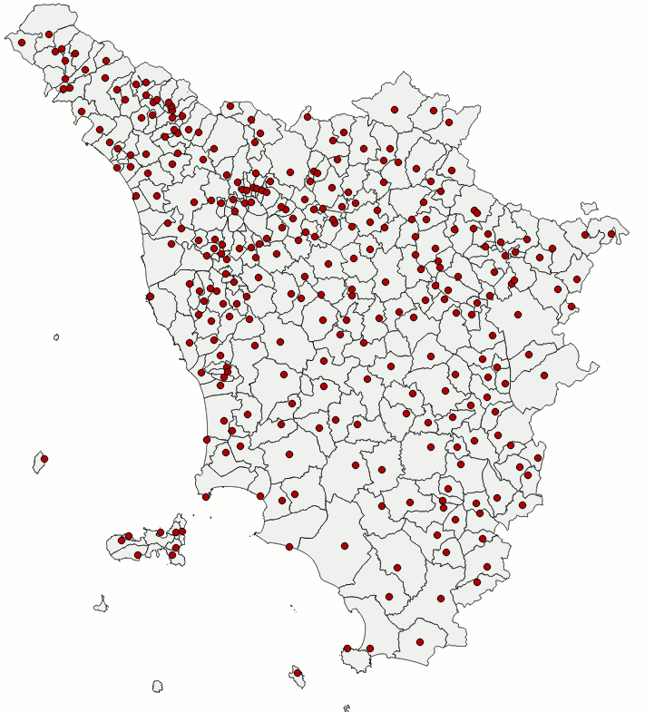
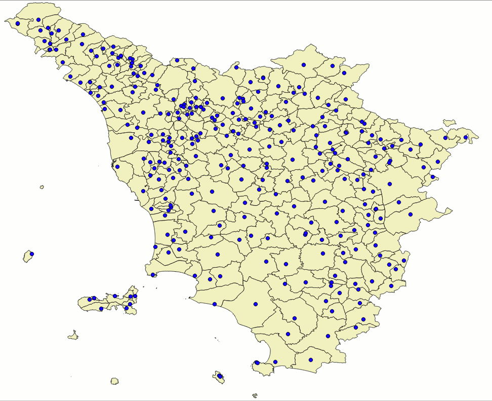
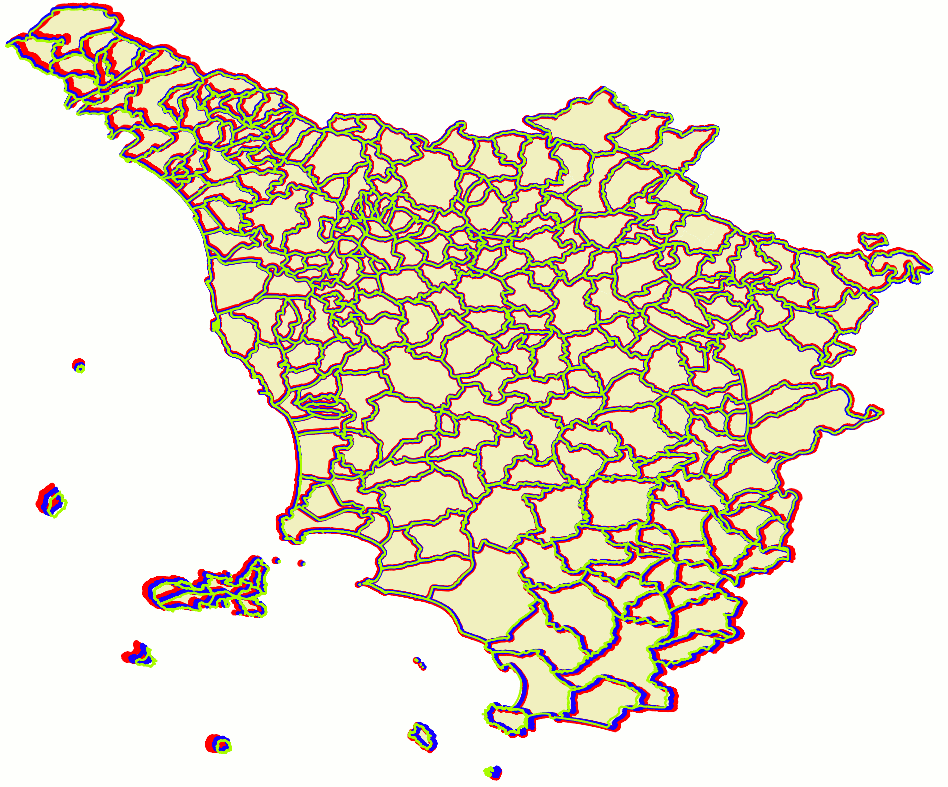
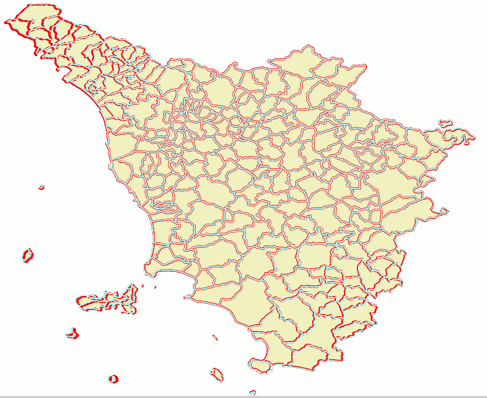
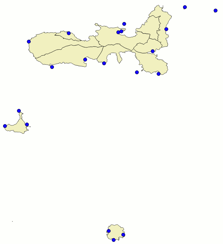
Imagine two different maps obviously representing the same identical geographic area, as the two shown on the side. Now suppose that only in one case the Coordinate Reference System is well known and fully qualified; however (for any good reason) the other map is completely lacking any useful information about its own CRS. You could be legitimately interested in merging together both maps, anyway this operation seems to be completely forbidden simply due to the complete lack of critical informations about one of the two maps. In this specific case adopting the usual coordinate transformations based on PROJ.4 and ST_Transform() is completely out of discussion. Just to say, this is the usual condition of many potentially interesting historical maps; but in many others cases too it frequently happens to encounter some odd map based on a completely undocumented CRS. Other times it could be a well known CRS unhappily unsupported by the standard EPSG geodetic definitions simply because it's based on some extravagant or not very common projection system completely unfit to match the standard EPSG expectations (an infamous example surely familiar to many Italian readers is represented by the Cassini-Soldner projection widely adopted by the Italian National Cadastre). Well, in all these cases the GCP approach can successfully resolve all your problems in a rather simple way. Let's see how it practically works:
You can now download the sample dataset we'll use in the following practical examples.
SELECT org.name, org.geometry, dst.geometry
FROM unknown_ppl AS org, geonames_ppl AS dst
WHERE Upper(org.name) = Upper(dst.name);
As you can easily check by executing the above SQL query, the Populated Places could be effectively used so to automatically create a set of 269 GCP pairs. We cannot probably expect an hi-quality result starting from a raw collection of unchecked data, but that's certainly enough to immediately start a first test session. Let's go on.
| |
|
First attempt and SQL familiarization
|
CREATE TABLE tuscany_1st AS
SELECT u.name, GCP_Transform(u.geometry, g.matrix, 4326) AS geometry
FROM unknown AS u,
     (SELECT GCP_Compute(org.geometry, dst.geometry) AS matrix
      FROM unknown_ppl AS org, geonames_ppl AS dst
      WHERE Upper(org.name) = Upper(dst.name)) AS g;

SELECT RecoverGeometryColumn('tuscany_1st', 'geometry', 4326, 'MULTIPOLYGON', 'XY');
|
CREATE TABLE tuscany_2nd AS
SELECT u.name, GCP_Transform(u.geometry, g.matrix, 4326) AS geometry
FROM unknown AS u,
     (SELECT GCP_Compute(org.geometry, dst.geometry, 2) AS matrix
      FROM unknown_ppl AS org, geonames_ppl AS dst
      WHERE Upper(org.name) = Upper(dst.name)) AS g;

SELECT RecoverGeometryColumn('tuscany_2nd', 'geometry', 4326, 'MULTIPOLYGON', 'XY');
| |
CREATE TABLE tuscany_3rd AS
SELECT u.name, GCP_Transform(u.geometry, g.matrix, 4326) AS geometry
FROM unknown AS u,
     (SELECT GCP_Compute(org.geometry, dst.geometry, 3) AS matrix
      FROM unknown_ppl AS org, geonames_ppl AS dst
      WHERE Upper(org.name) = Upper(dst.name)) AS g;

SELECT RecoverGeometryColumn('tuscany_3rd', 'geometry', 4326, 'MULTIPOLYGON', 'XY');
| |
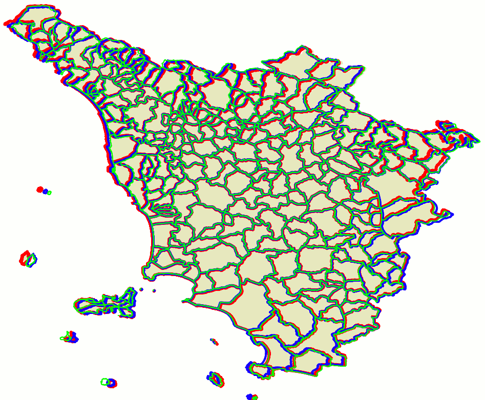
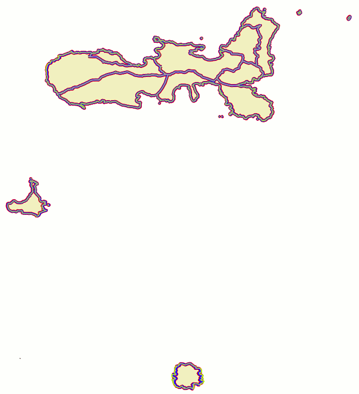
results assessmentThe side figure is a visual representation of the above SQL queries:
As you can easily notice, this first results are surely encouraging (they directly confirm that we are proceeding in the right direction), anyway they certainly suffer from many obvious problems.
Lesson learnt: GCP can surely produce better results than this, but now it's absolutely evident that accurately defining a good set of valid GCP pairs is a demanding and time consuming task. Accuracy and precision of input GCP pairs have a big impact on the final result quality. |
|
second attempt: using selected hi-quality GCP pairs
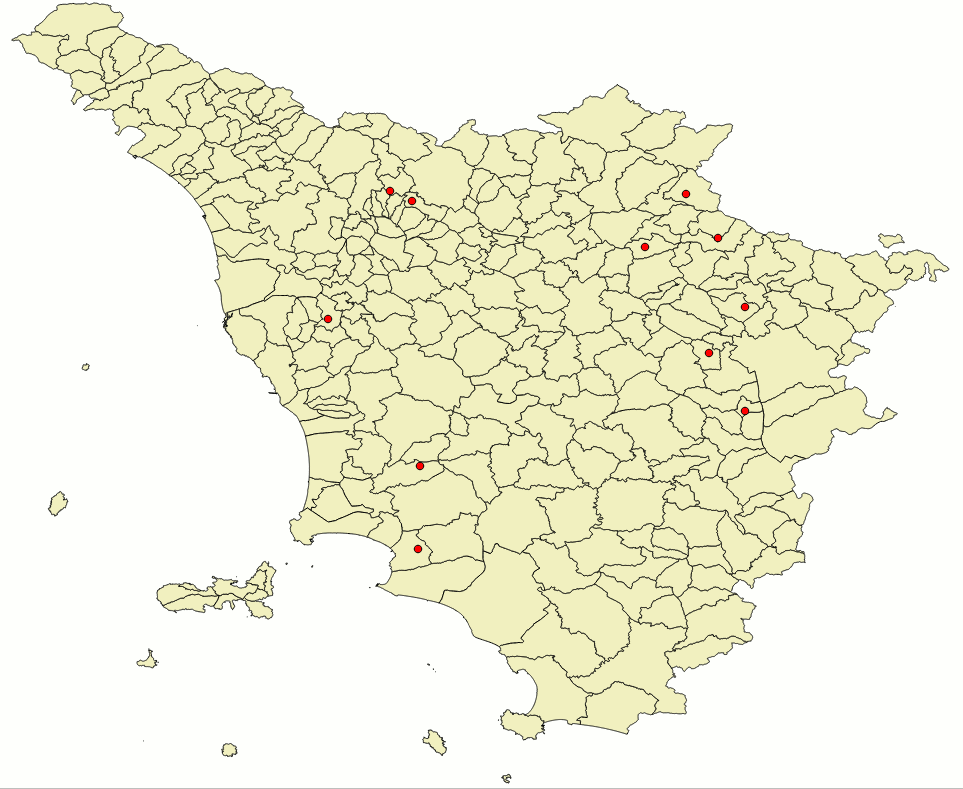
SELECT org.name, org.geometry, dst.geometry
FROM unknown_ppl AS org, geonames_ppl AS dst
WHERE dst.selected = 1 AND Upper(org.name) = Upper(dst.name);
As you can easily check by yourself the geonames_ppl dataset includes a selected column containing BOOLEAN values; the intended scope is to allow filtering a limited set of points presenting a very strict correspondence with their mates on the other map.
CREATE TABLE tuscany_bis_3rd AS
SELECT u.name, GCP_Transform(u.geometry, g.matrix, 4326) AS geometry
FROM unknown AS u,
     (SELECT GCP_Compute(org.geometry, dst.geometry, 3) AS matrix
      FROM unknown_ppl AS org, geonames_ppl AS dst
      WHERE dst.selected = 1 AND Upper(org.name) = Upper(dst.name)) AS g;

SELECT RecoverGeometryColumn('tuscany_bis_3rd', 'geometry', 4326, 'MULTIPOLYGON', 'XY');
So you can now duly repeat the same SQL queries as above just introducing few changes so to restrict the GCP selection to this hi-quality subset.The side figure graphically shows the position of such selected points; as you can notice they present a sub-optimal distribution, because they just cover the central portion of the map leaving many peripheral areas completely uncovered. |
|
results assessmentWe'll use the same colour schema we've already adopted in the previous test:
As the top side figure shows we've now a noticeably increased overall quality. Many obvious issues still affects the most peripheral areas of the map, anyway there is a significant enhancement on a wider central area. The bottom side figure shows a comparison of 2nd order and TPS transformations (in the previous test TPS was unable to resolve the GCP problem due to the poor quality of input data). It's interesting noting that TPS too produces very similar results to the ones produced by the 2nd order polynomial transformation. Lesson learnt: using a limited number of accurately selected hi-quality GPCs can easily produce better results than using a huge number of poorly defined GCPs. |
|
|
|
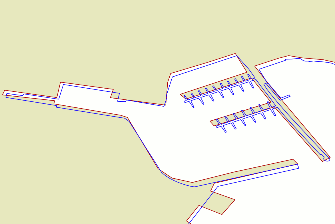
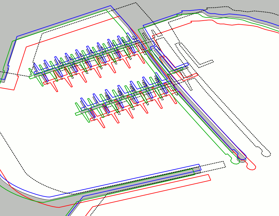
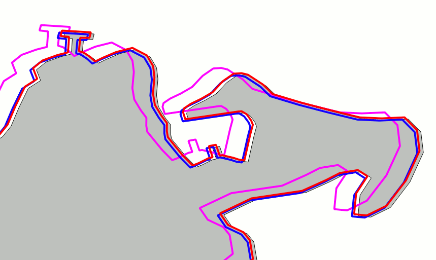
Quality assessmentThe top side figure directly compares the tuscany and the unknown datasets; the second dataset has been reprojected into SRID=4326 via ST_Transform().The scene corresponds to a barge pier in the harbour of Portoferraio (Elba Island). As you can notice the two datasets are noticeably different under many aspects, and several fine details are represented in a completely different way. This is absolutely not surprising, once considered that:
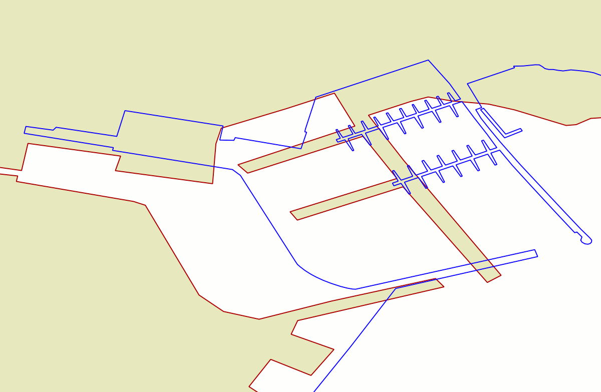
The bottom side figure represent the same area, but in this case the blue line corresponds to the result of the 2nd order polynomial transformation. At this representation scale it's absolutely obvious that there is a noticeable position error. Our efforts to use a GCP approach so to make the two datasets to spatially coincide still is someway unsatisfactory. We are absolutely required to identify a better strategy producing higher quality results. |
|
final attempt: separately processing a smaller sub-sample and wisely placing hi-quality GCP pairs
|
In this last exercise you are expected to download a further sample dataset; it simply contains a reduced sub-sample just covering the Elba Island, the Pianosa Island and the Montecristo Island. As shown in the side figure, we'll then proceed by using a more realistic set of control points; this time 20 GCPs have been carefully identified on both maps accordingly to the following criteria:
The names of the Shapefiles are exactly the same adopted in our fist example, so you can directly create a new DB-file by simply recycling the same SQL statements we have already used before without applying any change. |
|
results assessmentWe'll use the same colour schema we've already adopted in the previous tests:
As the side figure shows we've now a fairly good quality. Just in the case of the Montecristo Island (the southern one) we can notice at first glance some evident symptoms of a someway imperfect overlapping condition. This is not too much surprising, because Montecristo is not very closely related to other two islands, Adopting an even more restricted sub-sample could probably help in order to overcome these latest issues; anyway we can surely appreciate a noticeable overall improvement. |
|
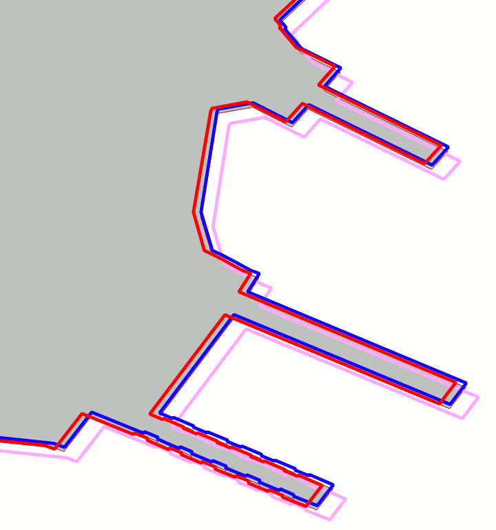
Quality assessment
Both 2nd order and TPS seems to be on par, and we finally have an hi-quality transformation affected by very reduced approximation errors. The 1st order give us a decent but clearly inferior result; the 3rd order surely is the less attractive of them all. |
 Portoferraio harbour - Barge piers |
A quick check on different areas of the map confirms the above reported general trends.
Both 2nd order and TPS transformations are roughly equivalent and produce hi-quality results. It's worth noting that both methods present a strong mutual consistency. The 1st order transformation is clearly affected by several troubles. |
 Portoferraio harbour - Ferry piers |
 Pianosa Island - Harbour |
Boring SQL functions: a formal introduction
| SQL Function | Description |
|---|---|
| GCP_Transform ( BLOB Geometry , BLOB GCP-coeffs ) : BLOB Geometry | Will return a new Geometry by applying a Polynomial or TPS Transformation to the input Geometry. The output Geometry will preserve the original SRID, dimensions and type. NULL will be returned on invalid arguments. |
| GCP_Transform ( BLOB Geometry , BLOB GCP-coeffs , int srid ) : BLOB Geometry | Same as above, but the output Geometry will assume the explicitly set SRID. |
| GCP_IsValid ( BLOB GCP-coeffs ) : BOOLEAN | Will check if a BLOB do really correspond to encoded GCP-coeffs then returning TRUE or FALSE. -1 will be returned if the argument isn't of the BLOB type. |
| GCP_AsText ( BLOB GCP-coeffs ) : TEXT | Will return a text serialized representation of the GCP-coeffs. NULL will be returned on invalid arguments. |
| GCP_Compute ( BLOB GeometryA , BLOB Geometry B ) : BLOB GCP-coeffs GCP_Compute ( BLOB GeometryA , BLOB GeometryB , int order) : BLOB GCP-coeffs |
Will return a BLOB-encoded set of coefficients representing the solution of a GCP problem. NULL will be returned on invalid arguments.
Aggregate function |
| GCP2ATM ( BLOB GCP-coeffs ) : BLOB ATM-matrix | Will convert a BLOB GCP-coeffs object into a BLOB-encoded Affine Transformation Matrix. NULL will be returned on invalid arguments. This function only accepts an argument corresponding to a set of polynomial coeffs of the 1st order. Note: only a polynomial transformation of the first order is mathematically equivalent to an Affine Transformation Matrix. |
Credits
The GCP module internally implemented by libspatialite fully depends on C code initially developed for GRASS GIS, and more precisely on the low-level sources implementing the v.rectify operator.SpatiaLite itself simply implements a thin layer of SQL compatibility, but beyond the scenes all the hard mathematical and statical work is completely delegated to the routines kindly borrowed by GRASS GIS.
The advantages of such a solution are rather obvious:
- avoiding to reinvent the wheel yet another time.
- taking full profit from reusing already existing code coming from a well renown source of indisputable excellence.
License considerations
The C code borrowed from GRASS GIS was initially released under the GPLv2+ license terms.Due to the intrinsic viral nature of GPL by enabling the GCP module you'll automatically cause libspatialite as a whole to fall under the GPLv2+ license legal terms.
There is no contradiction in all this: as the SpatiaLite's own license verbatim states:
SpatiaLite is licensed under the MPL tri-license terms; you are free to choose the best-fit license between:
    the MPL 1.1
    the GPL v2.0 or any subsequent version
    the LGPL v2.1 or any subsequent version
by enabling the GCP module you'll then automatically opting for the "GPL v2.0 or any subsequent version" legal clause.If you eventually would wish better to fully preserve the unconstrained initial tri-license you simply have to completely disable the GCP module when configuring libspatialite itself.
The default setting always corresponds to ./configure --enable-gcp=no: so you necessarily have to express an explicit consent in order to trigger the mandatory GPLv2+ license terms.
Back to main 4.3.0 Wiki page