Note: these pages are no longer maintained

Never the less, much of the information is still relevant.
Beware, however, that some of the command syntax is from older versions, and thus may no longer work as expected.
Also: external links, from external sources, inside these pages may no longer function.

	Recipe #1: Creating a well designed DB
2011 January 28

Previous Slide

Table of Contents

Next Slide

Normal Form

Any well designed DB adheres to the relational paradigm, and implements the so-called Normal Form.
Very simply explained in plain words:

you'll first attempt to identify any distinct category (aka class) present into your dataset
and simultaneously you have to identify any possible relation connecting categories.
data redundancy is strongly discouraged, and has to be reduced whenever is possible.

Consider the ISTAT Census 2001; identifying categories and relations is absolutely simple:

At the lowermost hierarchy level we have obviously Local Councils.
Each Local Council surely belongs to some County: so a relation exists connecting Local Councils and Counties.
To be more descriptive, this one is a typical one-to-many relationship
(one single County / many Local Councils: placing the same Local Council on two different Counties is absolutely forbidden).
The same is true for Counties and Regions.
There is not real need to establish a relation between Local Councils and Regions, because we can get this relation using the County as an intermediate pivot.

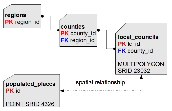
Accordingly to this, it's quite easy to identify several flaws in the original Shapefile's layout:

a POP2001 value is present for Local Councils, Counties and Regions:
well, this one clearly is an unneeded redundancy.
We simply have to preserve this information at the lowermost level (Local Councils):
because we can then compute anyway an aggregate value for Counties (or Regions).
a second redundancy exists: there is no real need compelling us to store both County and Region codes for each Local Council.
Preserving the County code is just enough, because we can get a reference to the corresponding Region anyway simply referencing the County.
a Geometry representation is stored for each County and Region:
this too represents an unneeded redundancy, because we can get such Geometries simply aggregating the ones stored at the Local Council level.

Then we have the cities1000 dataset: which comes from a completely different source (so there is no useful key we can use to establish relations to other entities).
And this dataset is in the 4326 SRID (WGS84), whilst any ISTAT - Census 2001 dataset is in the 23032 SRID [ED50 UTM zone 32];
so for now will simply keep this dataset in a completely self-standing state.
We'll see later how we can actually integrate this dataset with the other ones: after all, all them represent Italy, isn't ?
For sure some geographic relationship must exist ...

CREATE TABLE regions (
region_id INTEGER NOT NULL PRIMARY KEY,
region_name TEXT NOT NULL);

Step 1a) we'll start creating the regions table (i.e. the one positioned at the topmost hierarchic level).
Please note: we have defined a PRIMARY KEY, i.e. a unique (not duplicable), absolutely unambiguous identifier for each Region.

INSERT INTO regions (region_id, region_name)
SELECT COD_REG, REGIONE
FROM reg2001_s;

Step 1b) then we'll populate the regions table.
Using the INSERT INTO ... SELECT ... is more or less like performing a copy:
rows are extracted from the input table and immediately inserted into the output table.
As you can see, corresponding columns are explicitly identified by order.

CREATE TABLE counties (
  county_id INTEGER NOT NULL PRIMARY KEY,
  county_name TEXT NOT NULL,
  car_plate_code TEXT NOT NULL,
  region_id INTEGER NOT NULL,
  CONSTRAINT fk_county_region
    FOREIGN KEY (region_id)
    REFERENCES regions (region_id));

INSERT INTO counties (county_id, county_name,
car_plate_code, region_id)
SELECT cod_pro, provincia, sigla, cod_reg
FROM prov2001_s;

Step 2a) we'll now create (and populate) the counties table.
Please note: a relation exists linking counties and regions.
Defining an appropriate FOREIGN KEY we'll make such relation to be explicitly set once for all.

CREATE INDEX idx_county_region
ON counties (region_id);

Step 2b) accordingly to performance considerations, we must also create an INDEX corresponding to each FOREIGN KEY we'll define.

Very shortly explained: a PRIMARY KEY isn't simply a logical constraint.
In SQLite defining a PRIMARY KEY automatically implies generating an implicit index supporting fast direct access to each single row.
But on the other side defining a FOREIGN KEY simply establishes a logical constraint:
so if you actually wish to support fast direct access to each single row you have to explicitly create the corresponding index.

CREATE TABLE local_councils (
  lc_id INTEGER NOT NULL PRIMARY KEY,
  lc_name TEXT NOT NULL,
  population INTEGER NOT NULL,
  county_id INTEGER NOT NULL,
  CONSTRAINT fk_lc_county
    FOREIGN KEY (county_id)
    REFERENCES counties (county_id));

CREATE INDEX idx_lc_county
ON local_councils (county_id);

Step 3a) we'll now create the local_councils table.
A relation exists linking local_councils and counties.
So in this case too we have to define a FOREIGN KEY , then creating the corresponding index.
Please note: we haven't defined any Geometry column, although one is required for local_councils;
this is not a mistake, this is absolutely intentional.

SELECT AddGeometryColumn(
'local_councils', 'geometry',
23032, 'MULTIPOLYGON', 'XY');

Step 3b) creating a Geometry column isn't the same as creating any other ordinary column.
We have to use the AddGeometryColumn() spatial function, specifying:

the table name
the geometry column name
the SRID to be used
the expected geometry class
the dimension model
(in this case, simple 2D)

INSERT INTO local_councils (lc_id,
lc_name, population, county_id, geometry)
SELECT PRO_COM, NOME_COM, POP2001,
COD_PRO, Geometry
FROM com2001_s;

Step 3c) after all this can populate the local_councils table as usual.

CREATE TABLE populated_places (
  id INTEGER NOT NULL
    PRIMARY KEY AUTOINCREMENT,
  name TEXT NOT NULL);

SELECT AddGeometryColumn(
'populated_places', 'geometry',
4326, 'POINT', 'XY');

INSERT INTO populated_places (id,
name, geometry)
SELECT NULL, COL002,
MakePoint(COL006, COL005, 4326)
FROM cities1000
WHERE COL009 = 'IT';

Step 4) you have now to perform the last step: creating (and populating) the populated_places table.
Several interesting points to be noted:

we have used an AUTOINCREMENT clause for the PRIMARY KEY
this practically means that SQLite can automatically generate an appropriate unique value for this PRIMARY KEY, when no explicit value has been already set.
accordingly to this, in the INSERT INTO statement a NULL value was set for the PRIMARY KEY:
and this explicitly solicited SQLite to assign automatic values.
the original cities1000 dataset shipped two numeric columns for longitude [COL006] and latitude [COL005]:
so we have to use the MakePoint() Spatial function in order to build a point-like Geometry.
using the SRID 4326 we set such Geometry into the WGS84 [Geographic System] SRS.

Just to recapitulate:

You started this tutorial using Virtual Shapefiles (and Virtual CSV/TXT) tables.
Such Virtual Tables aren't at all real DB tables: they aren't internally stored.
They simply are trivial external files accessed using an appropriate driver.
Using Virtual Tables at first allowed you to test some simple and very basic SQL queries.
But in order to test more complex SQL features any dataset have to be properly imported into the DBMS itself.
And this step required creating (and then populating) internal tables, accordingly to a well designed layout.

DROP TABLE com2001_s;
DROP TABLE prov2001_s;
DROP TABLE reg2001_s;
DROP TABLE cities1000;

Step 5) and finally you can drop any Virtual Table, because they aren't any longer useful.
Please note: dropping a Virtual Shapefile or Virtual CSV/TXT doesn't removes the corresponding external data-source, but simply removes the connection with the current database.

Previous Slide

Table of Contents

Next Slide

	Author: Alessandro Furieri a.furieri@lqt.it
	This work is licensed under the Attribution-ShareAlike 3.0 Unported (CC BY-SA 3.0) license.

	Permission is granted to copy, distribute and/or modify this document under the terms of the GNU Free Documentation License, Version 1.3 or any later version published by the Free Software Foundation; with no Invariant Sections, no Front-Cover Texts, and no Back-Cover Texts.