Quick How-To Guide for the Planet Earth sample

In this tutorial we'll assume that you've already studied and understood the tutorials about the Giglio sample
Now we'll examine the Planet Earth sample which will allow us to delve further into new details that we previously ignored.

The following table summarizes for quick reference all Coverages contained into the Planet Earth sample database:

Coverage name	Type	Description
etopo1	Raster	Global DEM - Digital Elevation Model
true_marble	Raster	Natural colors - RGB low-resolution mosaic of Landsat imagery
countries	Vector	2D Polygons - National Boundaries
countries_vw	Vector	Spatial View derived from countries
topo_states	Vector	Topology derived from countries

All datasets are based on open data available at the following URLs:

ETOPO1: NOAA
True Marble: Unearthed Outdoors
Countries: Natural Earth

Step #1 - General Introduction

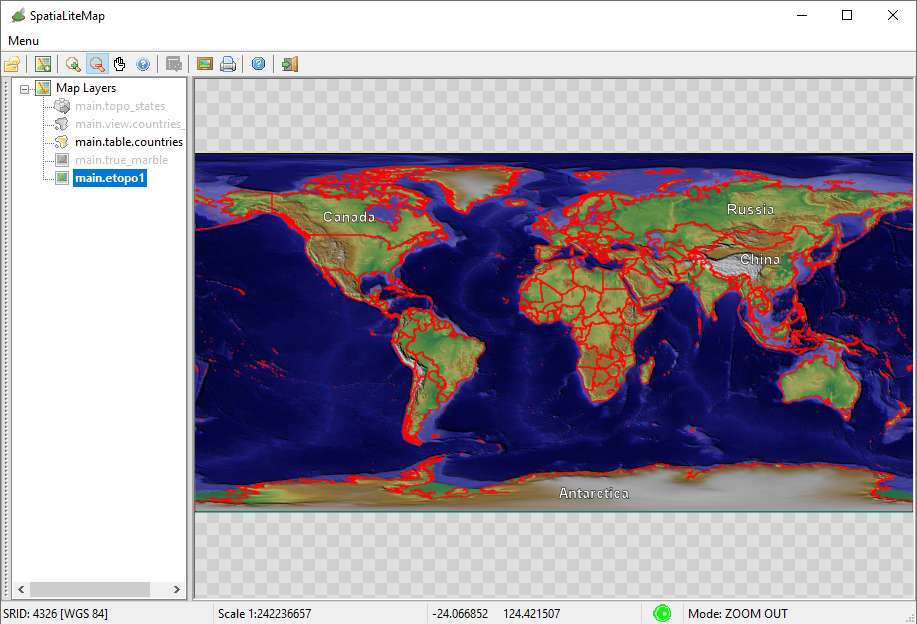
In this first contact with Planet Earth we'll simply test the basic rendering capabilities of the Map.

You are simply expected to test the pan and zoom tools while switching on and off the various map layers.

Step #1.1 - Testing the ETOPO1 background

The side figure shows how the Map will be when applying the following layers selection:

ETOPO1 background
Countries (National Boundaries - red lines) with labels corresponding to each Nation.
- Note: labels will be printed only if they fit inside the MBR of the corresponding Polygon

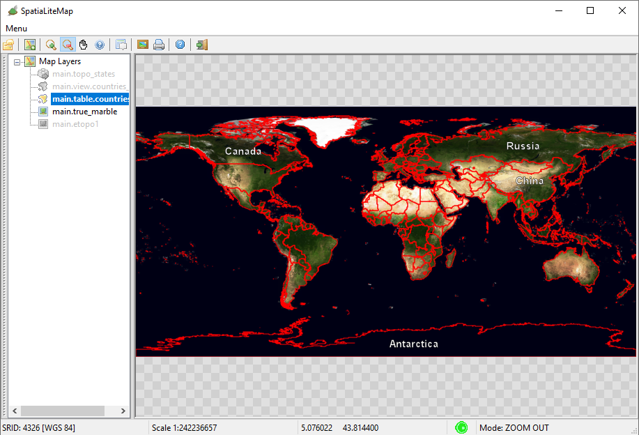
Step #1.2 - Testing the True Marble background

The side figure shows how the Map will be when applying the following layers selection:

True Marble background
Countries (same as above).

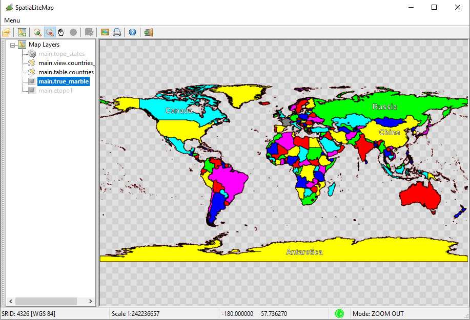
Step #1.3 - Testing the Political Map

The side figure shows how the Map will be when applying the following layers selection:

Countries (view) background
- Note: Each Country is internally filled with a different color, in such a way that confining Nations will never share the same color.
Countries (same as above).

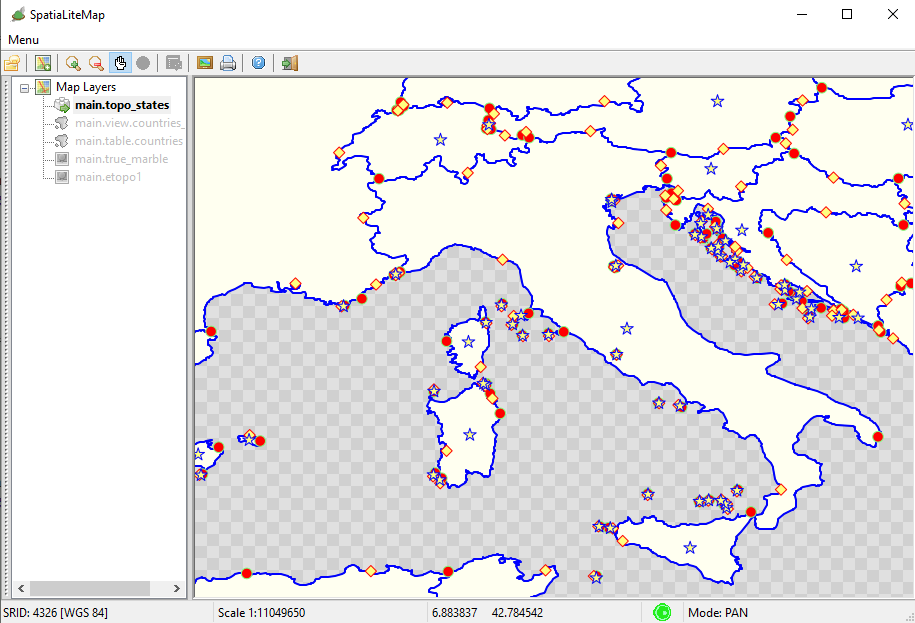
Step #1.4 - Testing the Topology

The side figure shows how the Map will be when applying the following layers selection:

topo_states (Topology) alone. All Topology Primitives are represented as follows:
- Nodes: red circles.
- Edges: blue lines.
- Faces: pale yellow polygons.
- Face Seeds: yellow stars.
- Edge Seeds: yellow diamonds.

Step #2 - Preparing the Raster Coverages

Step #2.1 - Creating the Raster Coverages

Useful hint

Both etopo1 and true_marble will be imported from a single GeoTiff. Using the tiffinfo CLI tool so to check the internal configuration of the input images is warmly recommended.

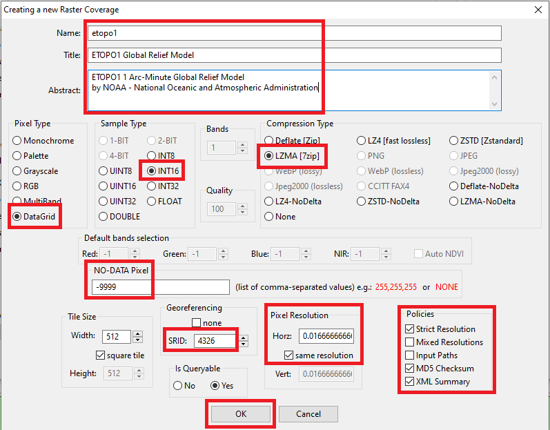
Step #2.1.1 - Creating etopo_1

Set sensible values tof Name, Title and Abstract.
This one is a DEM, and the most appropriate settings are as follows:
- Pixel Type set to DataGrid
- Sample Type set to INT16
- Compression Type set to LZMA
- NO-DATA set to -9999
- SRID set to 4326
- Pixel Resolution set to 0.016666...
- The Strict Resolution Policy has been selected.

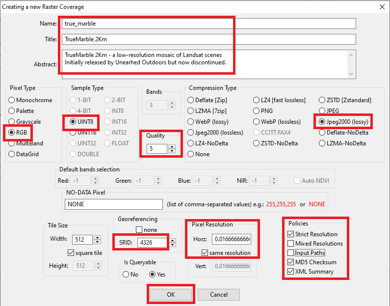
Step #2.1.2 - Creating true_marble

Set sensible values tof Name, Title and Abstract.
This one is a RGB image, so the most appropriate settings are as follows:
- Pixel Type set to RGB
- Sample Type set to UINT8
- Compression Type set to JPEG2000 (because it's a rather slow codec, but it preserves a good visual quality at very high compression ratios).
- Quality set to 5 (so to ensure a very good compression ratio without sacrificing too much the visual quality).
- NO-DATA set to NONE
- SRID set to 4326
- Pixel Resolution set to 0.016666...
- The Strict Resolution Policy has been selected.

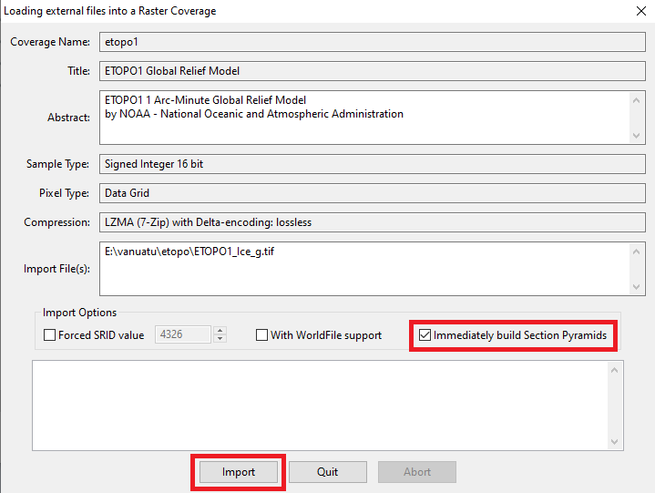
Step #2.2 - Populating the Raster Coverages

On the dialog box:

Remember to enable the Immediately build Section Pyramids checkbox

This recipe is valid for both etopo1 and true_marble

Note: in this case you should absolutely avoid to select the Forced SRID value and/or With WorldFile support checkbox because we are importing from GeoTiff that internally stores any required information.

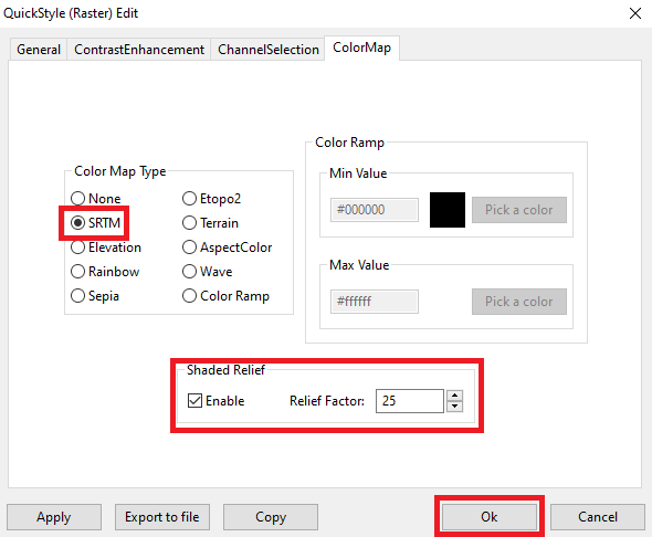
Step #2.3 - Styling the Raster Coverages

etopo1 is Global DEM, presenting elevation values ranging between the ocean depths and the very high peaks of the Himalayas.
The most appropriate choice for the Color Map Style could be either Etopo2 or SRTM or Terrain.

Note: setting up a Style for true_marble is not required, because this one is a RGB Coverage, and the default Style will be perfectly adequate.

Step #3 - Preparing the Vector Coverages

Step #3.1 - Styling countries (Spatial Table)

This recipe is valid for both etopo1 and true_marble

There is very little to say about creating and populating the countries Spatial Table, because we'll just import the Shapefile downloaded from Natural Earth.

Then transforming this Spatial Table into a corresponding Vector Coverage should be a trivial task; if you have doubts about this passage you just have to return to the previous tutorial.

So we'll focus out attention just on the Style, that is a little bit more elaborate then usual.

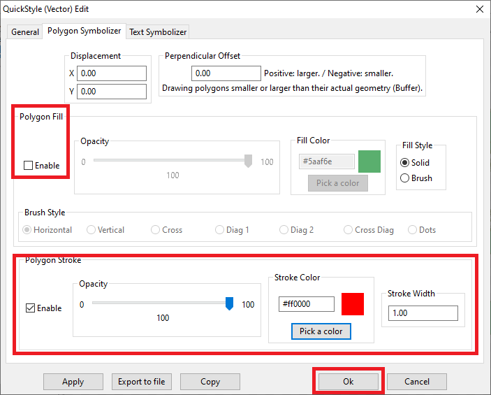
Step #3.1.1 - Setting up the Polygon Symbolizer

On the QuickStyle Dialog Box:

open the Polygon Symbolizer tab.
be sure to disable the Fill option.
enable the Stroke option.
- Note: this way we'll get hollow polygons, completely lacking any internal filling, so to preserve fully visible the underlaying Raster.
and finally press the Ok button so to confirm.

We've not yet finished.
Now we'll add a second Symbolizer to the current Style, and it will exactly be a Text Symbolizer

This way each polygon will have the name of the corresponding Nation printed on its surface.

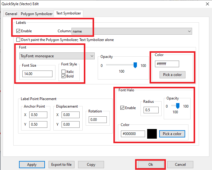
Step #3.1.2 - Setting up the Text Symbolizer

On the QuickStyle Dialog Box:

open the Text Symbolizer tab.
be sure to enable the Labels option.
select from the list the name of the Column containing the values to printed as labels (in this case name).
Choose some Font from the list
- Note: all fonts accessible to RasterLite2 must be stored into the SE_fonts table.
  You'll find some user friendly wizards making easier handling Fonts in the context menu associated to the Styling (SLD/SE) node on the Tree Control.
  Few Toy Fonts are always available because they are directly embedded in the code.
Set an appropriate Font Size and select the Bold option for better readability.
Enable the Font Halo option and specifiy a very thin Radius
- Note: for what concerns Colors we've set white text surrounded by a narrow black halo so to unsure a good readability on every background.
and finally press the Ok button so to confirm.

Step #3.2 - Creating and styling a Vector Coverage based on a Spatial View

Step #3.2.1 - Creating the Spatial View

There is very little to say about this; we simply have to execute a pair of SQL statements.

What is decisely more interesting to be examined is the intended role of the CASE clause:

if you quicly examine the countries table you'll discover the presence of a Column named mapcolor7
as you can easily check, all values in this column range from 1 to 7
Short conclusion: that mapcolor7 column is specifically intended to contain color indices allowing to easily style a Political Map of the World.
So in our View we simply have to transform each color index into a corresponding HTML hex color, and exactely this is the intended scope of the CASE clause.

CREATE VIEW countries_vw AS
SELECT pk_uid AS rowid, name AS name,
    CASE mapcolor7
        WHEN 1 THEN '#FF0000'
        WHEN 2 THEN '#00FF00'
        WHEN 3 THEN '#0000FF'
        WHEN 4 THEN '#FFFF00'
        WHEN 5 THEN '#FF00FF'
        WHEN 6 THEN '#00FFFF'
        ELSE '#808080'
    END color, geometry AS geom
FROM countries;

INSERT INTO views_geometry_columns VALUES
    ('countries_vw', 'geom', 'rowid', 'countries', 'geometry', 1);

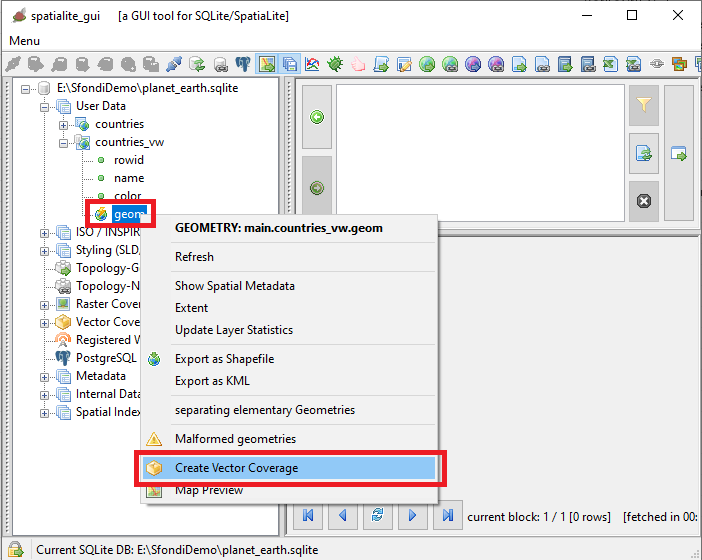
Step #3.2.2 - Transforming a Spatial View into a Vector Coverage

From the Tree View expand the Spatial View node, then go to its Geometry node:

press the mouse right button
a context menu will be displayed on the screen
Click the Create Vector Coverage menu item

Note: the Style we'll go to create is not directly supported by any wizard; it strictly requires to be hand-written.
Don't be afraid because it will be extremely simple and easy.

first of all use the QuickStyles wizard in order to create a generic Polygon symbolizer
then export the XML code into an external file.
and finally open a text editor whatsoever so to manually complete the Style.

Step #3.2.3 - Styling the countries_vw Vector Coverage

How to edit the XML template:

you'll start as usual by setting appropriate values to Name, Title and Abstract
now you just are required to set the fill parameter as @color@

<?xml version="1.0" encoding="UTF-8"?>
<PolygonSymbolizer version="1.1.0"
    xsi:schemaLocation="http://www.opengis.net/se http://schemas.opengis.net/se/1.1.0/Symbolizer.xsd"
    xmlns="http://www.opengis.net/se" xmlns:ogc="http://www.opengis.net/ogc"
    xmlns:xlink="http://www.w3.org/1999/xlink"
    xmlns:xsi="http://www.w3.org/2001/XMLSchema-instance"
    uom="http://www.opengeospatial.org/se/units/pixel">
    <Name>countries_col</Name>
    <Description>
        <Title>Countries - Political Map</Title>
        <Abstract>A Style setting its Fill color from a Column Value</Abstract>
    </Description>
    <Fill>
        <SvgParameter name="fill">@color@</SvgParameter>
        <SvgParameter name="fill-opacity">1.00</SvgParameter>
    </Fill>
    <Stroke>
        <SvgParameter name="stroke">#000000</SvgParameter>
        <SvgParameter name="stroke-opacity">1.00</SvgParameter>
        <SvgParameter name="stroke-width">1.00</SvgParameter>
        <SvgParameter name="stroke-linejoin">round</SvgParameter>
        <SvgParameter name="stroke-linecap">round</SvgParameter>
    </Stroke>
</PolygonSymbolizer>

Step #3.3 - Creating and styling a Vector Coverage based on a Topology

Useful hint

If you ignore absolutely everything about Topology perhaps it would be advisable that you read the documentation first.

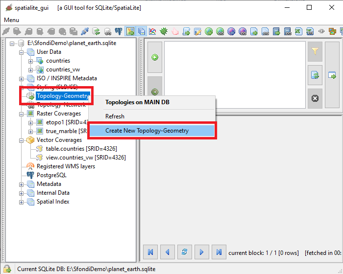
Step #3.3.1 - How to create a Topology

From the Topology-Geometry node in the Tree View:

press the mouse right button
a context menu will be displayed on the screen
Click the Create New Topology-Geometry menu item

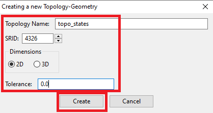
Step #3.3.2 - Creating the Topology

On the dialog box:

set a Topology Name
set an appropriate SRID
select 2D dimensions
set Tolerance to zero
and finally press the Create button in order to confirm

Step #3.3.3 - Building the Topology

There is very little to say, it just requires executing few SQL statements.

SELECT TopoGeo_FromGeoTableNoFaceExt('topo_states', NULL, 'countries', NULL, 'dustbin', 'dustbin_view', 512);

SELECT TopoGeo_Polygonize('topo_states'); 

SELECT TopoGeo_UpdateSeeds('topo_states');

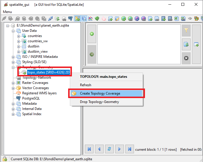
Step #3.3.4 - Transforming a Topology into a Vector Coverage

From the Topology-Geometry node in the Tree View:

expand the node so to make all Topologies visible
- from the child node corresponding to the intended Topology:
  - press the mouse right button
  - a context menu will be displayed on the screen
  - Click the Create Topology Coverage menu item

A Vector Coverage based on some Topology is someway exceptional, because it groups several different classes of Primitives:

Nodes
Edges
Faces
Face Seeds
Edge Seeds

Each one of them requires a specific Symbolizer.
All them will be switched on and off at the same time, because all them are considered as parts of the same layer.
Conclusion: the handling of Topology-based Coverages is someway exceptional, and requires special precautions.

Note: more or less the same applies to Network-based Coverages (that will not be illustrated in any tutorial).

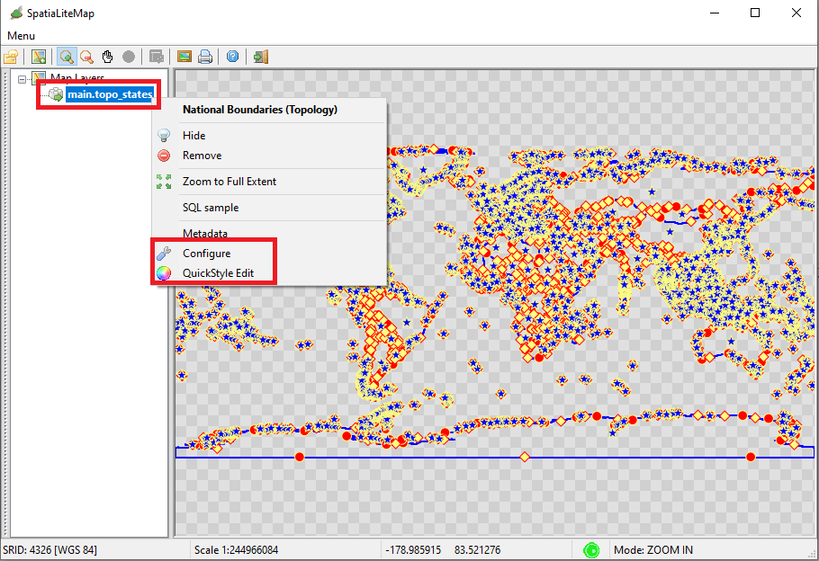
Step #3.3.5 - Handling a Topology-based Vector Coverage

From the main.topo_states node in the Tree View:

press the mouse right button
a context menu will be displayed on the screen
Both the Configure and QuickStyles Edit menu items influences the behavior of this Coverage

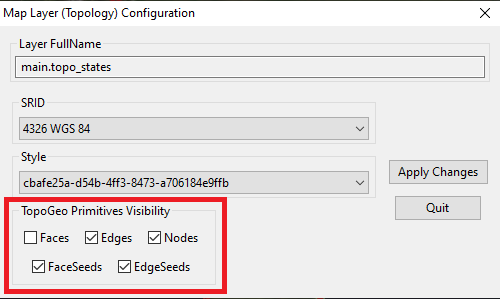
Step #3.3.6 - Handling the visibily of individual Topology Primitives

On the Configuration Dialog Box you can select / unselect the checkbox corresponding to each single Primitive
Any disabled Privitive class will never be shown on the Map.

Note: the Faces Primitive is usually kept disabled, because Topology Faces are simply virtual thus being very slow to be generated on the fly.
If the current viewpoint of the Map contains a reasonable number of Faces showing them could be acceptable.
But when the current viepoint contains a really huge number of Faces updating the Map will probably require an absolutely unacceptable time. You are warned, be very careful.

Step #3.3.7 - Styling a Topology-based Vector Coverage

Styling a Topology-based Coverage isn't at all difficult, it's just a little bit more complex than usual because you are required to define 5 different Symbolizers, one for each Primitive.
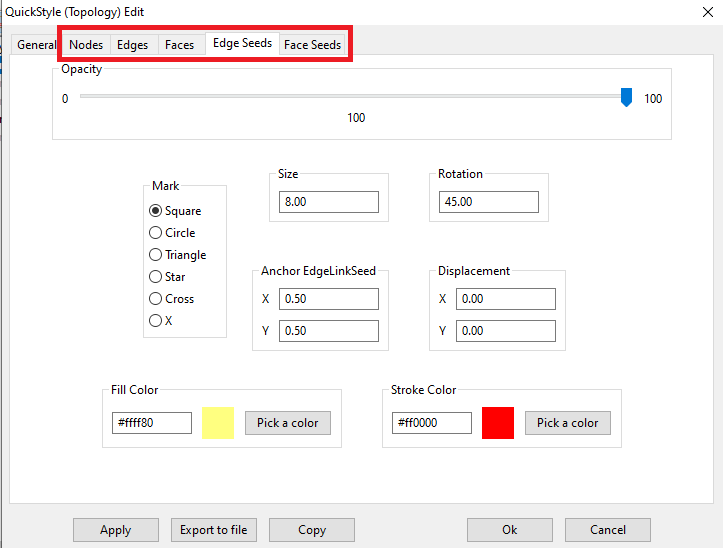