|
generic prototypes: ST_xxxxGrid( input Geometry, size double precision ) : grid Geometry ST_xxxxGrid( input Geometry, size double precision, edges_only boolean ) : grid Geometry ST_xxxxGrid( input Geometry, size double precision, edges_only boolean, origin Geometry ) : grid Geometry |
- the input Geometry is always expected to be a Polygon or a MultiPolygon, and will be exactly covered by the returned grid.
- the size argument identifies the edge length of the grid cell.
- the optional edges_only argument will be interpreted as follows:
- if FALSE (default value) a MultiPolygon will be returned.
- if TRUE a MultiLinestring will be returned (simply representing the cells edges).
- the optional origin Geometry is always assumed to be a Point, and will identify the grid's origin. By default a (0, 0) origin will be assumed.
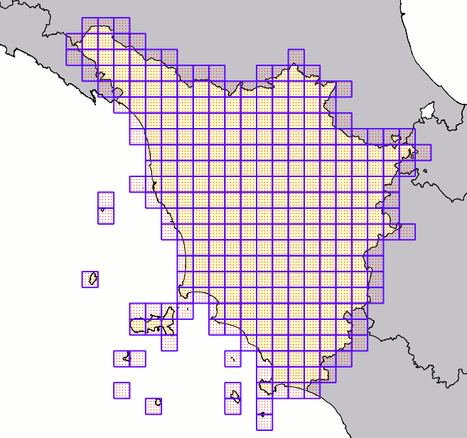
using Square cells
|
SELECT ST_SquareGrid(geometry, 10000) FROM regions WHERE cod_reg = 9; |
This SQL query will return a regular grid (square cells) covering Tuscany (cod_reg=9).
Each grid's cell will have an edge length of exactly 10 Km
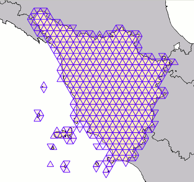
using Triangular cells
|
SELECT ST_TriangularGrid(geometry, 10000) FROM regions WHERE cod_reg = 9; |
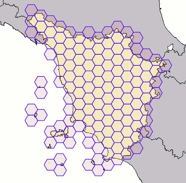
using Hexagonal cells
|
SELECT ST_HexagonalGrid(geometry, 10000) FROM regions WHERE cod_reg = 9; |